1D and 2D Dynamic Programming

The Five Concepts for Today

1. The 1D DP Pattern: Climbing Stairs
2. From 1D to 2D: Defining a Two-Dimensional State
3. Solving 2D DP: Longest Common Subsequence (LCS)
4. A Key 2D DP Variation: Edit Distance
5. Real-World Applications and Interview Strategy

Concept 1: The 1D DP Pattern: Climbing Stairs

This problem is a perfect reinforcement of the concepts from our last lesson. It's a classic 1D DP problem that shares a structure very similar to the Fibonacci sequence.

Problem: You are climbing a staircase. It takes n steps to reach the top. Each time you can either climb 1 or 2 steps. In how many distinct ways can you climb to the top?

Technical Explanation

Let dp[i] be the number of ways to reach the i-th step. To reach step i, you must have come from either step i-1 (by taking a single step) or step i-2 (by taking two steps). The total number of ways to reach step i is the sum of the ways to reach these two preceding steps. This gives us the recurrence relation:

This is the same recurrence as Fibonacci! The base cases are:

• dp[1] = 1 (one way to reach step 1: take one step)
• dp[2] = 2 (two ways to reach step 2: 1+1 or 2)

This structure, where the solution for dp[i] depends on a fixed number of immediately preceding states, is the hallmark of 1D DP.

Metaphor: An Assembly Line

Think of building a product on an assembly line with n stations. The state of the product at station i depends only on the work done at stations i-1 and i-2. To figure out the configuration at station i, you don't need to know what happened at station 1; you only need the recent history. The dp table is like a logbook, recording the state at each station, and you build it up sequentially from the start of the line.

Implementation

The path from a naive recursive solution to a space-optimized one is a journey you should be able to reconstruct. The following video walks through this entire process beautifully.

Here is the final, interview-ready Python code with space optimization.

def climb_stairs(n: int) -> int:
    """
    Calculates the number of ways to climb n stairs using a bottom-up
    approach with O(1) space.
    Time Complexity: O(n)
    Space Complexity: O(1)
    """
    if n <= 2:
        return n
    
    # prev2 stores ways(i-2), prev1 stores ways(i-1)
    prev2, prev1 = 1, 2
    
    for _ in range(3, n + 1):
        current_ways = prev1 + prev2
        prev2 = prev1
        prev1 = current_ways
        
    return prev1

print(f"Ways to climb 5 stairs: {climb_stairs(5)}") # Should be 8

Concept 2: From 1D to 2D: Defining a Two-Dimensional State

While 1D DP is powerful, many complex problems, especially those involving two strings or sequences, require a 2D state.

Technical Explanation

A 2D DP problem arises when a subproblem cannot be described by a single index. Instead, it needs two (or more) parameters to be uniquely identified. For problems comparing two strings, text1 and text2, a subproblem is typically about comparing a prefix of text1 with a prefix of text2.

We define a 2D table, dp[i][j], where:

• i corresponds to the length of the prefix of text1 (i.e., text1[0...i-1]).
• j corresponds to the length of the prefix of text2 (i.e., text2[0...j-1]).
• dp[i][j] stores the solution to the subproblem for these two prefixes.

The final solution to the original problem is usually found at dp[m][n], where m and n are the full lengths of the strings.

Metaphor: Filling a Spreadsheet

Imagine you have a spreadsheet where the rows are labeled with characters from text1 and columns with characters from text2. Filling out the cell at (row_i, col_j) requires you to look at the values in adjacent cells you've already filled: the one above (i-1, j), the one to the left (i, j-1), and the one diagonally up-left (i-1, j-1). You are systematically filling a grid, where each cell represents a more complex subproblem that depends on simpler, adjacent subproblems. Your final answer is in the bottom-right corner of the sheet.

Concept 3: Solving 2D DP - Longest Common Subsequence (LCS)

LCS is the canonical 2D DP problem. Given two strings, find the length of the longest subsequence present in both. A subsequence doesn't need to be contiguous. For example, "ace" is a subsequence of "abcde".

Technical Explanation

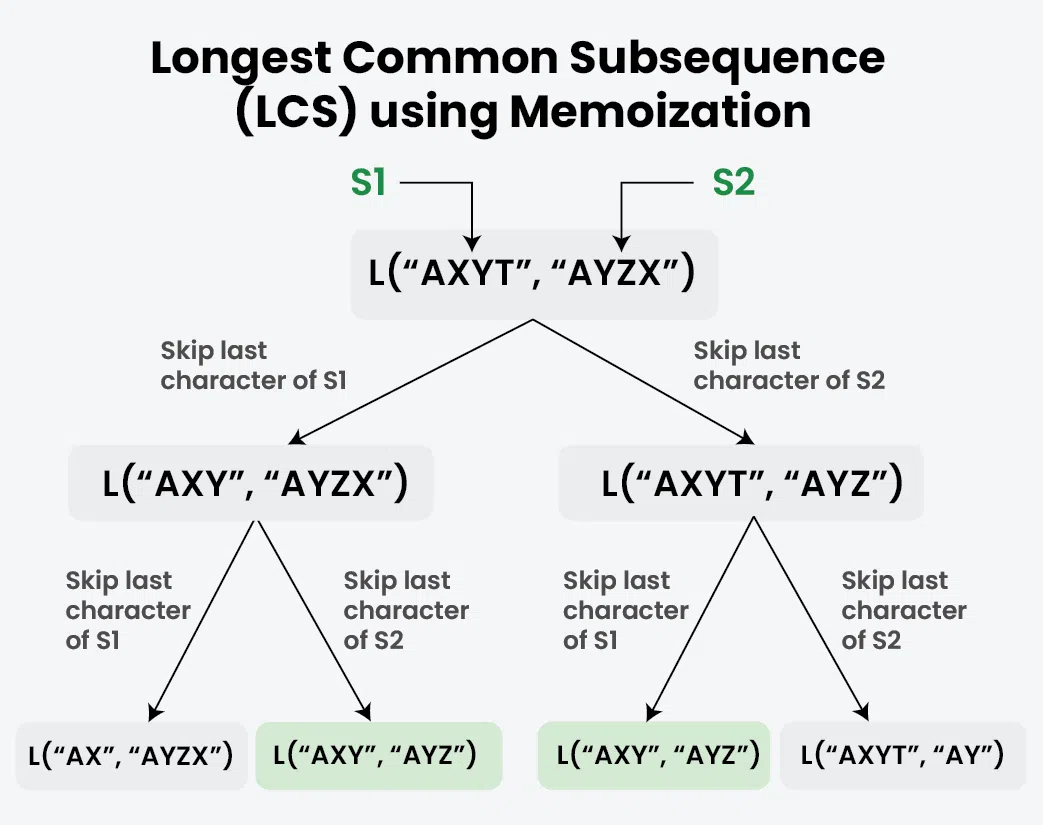
Let dp[i][j] be the length of the LCS of text1[:i] and text2[:j]. We build the (m+1) x (n+1) DP table by considering the characters text1[i-1] and text2[j-1].

There are two cases for the recurrence relation:

1. Characters Match: text1[i-1] == text2[j-1]
   If the characters match, they must be part of the LCS. We extend the LCS from the smaller subproblem dp[i-1][j-1].

   $$dp[i][j]=1+dp[i-1][j-1]$$

2. Characters Don't Match: text1[i-1] != text2[j-1]
   If they don't match, we can't use both. The LCS is the best we can do by either ignoring the character from text1 (and solving for text1[:i-1] and text2[:j]) or ignoring the character from text2 (and solving for text1[:i] and text2[:j-1]). We take the maximum of these two possibilities.

   $$dp[i][j]=\max (dp[i-1][j],dp[i][j-1])$$

The base cases are dp[i][0] = 0 and dp[0][j] = 0 for all i, j, as the LCS with an empty string is always 0.

Metaphor: DNA Sequence Alignment

Biologists use this exact logic to align two DNA strands. To find how similar two strands are, they slide them past each other.

• If the bases at the current position match (e.g., A and A), that's a point for the alignment score. They both advance to the next base. This is our 1 + dp[i-1][j-1] case.
• If the bases don't match (e.g., A and C), there's a "mismatch". The alignment algorithm has to decide whether to introduce a gap in the first strand or the second. It chooses whichever option leads to a better overall score down the line. This corresponds to our max(dp[i-1][j], dp[i][j-1]) case.

Implementation

The best way to understand the 2D DP table is to see it being filled.

Here's the bottom-up tabulated implementation.

def longest_common_subsequence(text1: str, text2: str) -> int:
    """
    Calculates the length of the longest common subsequence using 2D DP.
    Time Complexity: O(m * n)
    Space Complexity: O(m * n), where m and n are string lengths.
    """
    m, n = len(text1), len(text2)
    
    # dp[i][j] will be the LCS of text1[:i] and text2[:j]
    dp = [[0] * (n + 1) for _ in range(m + 1)]
    
    for i in range(1, m + 1):
        for j in range(1, n + 1):
            # Case 1: Characters match
            if text1[i-1] == text2[j-1]:
                dp[i][j] = 1 + dp[i-1][j-1]
            # Case 2: Characters do not match
            else:
                dp[i][j] = max(dp[i-1][j], dp[i][j-1])
                
    return dp[m][n]

print(f"LCS of 'abcde' and 'ace' is: {longest_common_subsequence('abcde', 'ace')}") # Expected: 3

Concept 4: A Key 2D DP Variation: Edit Distance

The Edit Distance (or Levenshtein Distance) problem is another 2D DP classic. It's very similar to LCS but has a slightly more complex recurrence.

Problem: Given two strings, word1 and word2, find the minimum number of operations (insert, delete, or replace) required to convert word1 to word2.

Technical Explanation

We again use a 2D table dp[i][j] to store the minimum edit distance between word1[:i] and word2[:j].

• Base Cases:

  • dp[i][0] = i: To convert a string of length i to an empty string requires i deletions.
  • dp[0][j] = j: To convert an empty string to a string of length j requires j insertions.

• Recurrence Relation:

  1. Characters Match: word1[i-1] == word2[j-1]
     If they match, no operation is needed. The cost is the same as the subproblem for the shorter prefixes.

     $$dp[i][j]=dp[i-1][j-1]$$

  2. Characters Don't Match: word1[i-1] != word2[j-1]
     We must perform one operation. We choose the one that results from the cheapest subproblem:

     • Insert: Convert word1[:i] to word2[:j-1] and then insert word2[j-1]. Cost: dp[i][j-1] + 1.
     • Delete: Convert word1[:i-1] to word2[:j] and then delete word1[i-1]. Cost: dp[i-1][j] + 1.
     • Replace: Convert word1[:i-1] to word2[:j-1] and then replace word1[i-1] with word2[j-1]. Cost: dp[i-1][j-1] + 1.

     We take the minimum of these three options:

     $$dp[i][j]=1+\min (dp[i][j-1],dp[i-1][j],dp[i-1][j-1])$$

Metaphor: Autocorrect

Think about how your phone suggests "algorithm" when you type "algorthm". It's calculating the edit distance!

• Match: 'a'=='a', 'l'=='l', ... no cost.
• Don't Match: When it sees 'h' where 'i' should be, it considers the options:
  • Replace: change 'h' to 'i' (1 op). Cost is cost("algort") -> "algor") + 1.
  • Delete: delete 'h', then try to match "algortm" with "algorithm" (1 op). Cost is cost("algort") -> "algorithm") + 1.
  • Insert: keep 'algorthm', insert 'i' and try to match "algorthm" with "algorithmi" (1 op). Cost is cost("algorthm") -> "algor") + 1.
    The system picks the cheapest path, which is a single replacement.

Implementation

def min_distance(word1: str, word2: str) -> int:
    """
    Calculates the minimum edit distance between two strings using 2D DP.
    Time Complexity: O(m * n)
    Space Complexity: O(m * n)
    """
    m, n = len(word1), len(word2)
    dp = [[0] * (n + 1) for _ in range(m + 1)]

    # Initialize base cases
    for i in range(m + 1):
        dp[i][0] = i
    for j in range(n + 1):
        dp[0][j] = j
    
    # Fill the DP table
    for i in range(1, m + 1):
        for j in range(1, n + 1):
            # Case 1: Characters match
            if word1[i-1] == word2[j-1]:
                dp[i][j] = dp[i-1][j-1]
            # Case 2: Characters don't match
            else:
                dp[i][j] = 1 + min(
                    dp[i-1][j],       # Deletion
                    dp[i][j-1],       # Insertion
                    dp[i-1][j-1]      # Replacement
                )
    
    return dp[m][n]

print(f"Edit distance between 'horse' and 'ros': {min_distance('horse', 'ros')}") # Expected: 3

Concept 5: Real-World Applications and Interview Strategy

Understanding these algorithms is one thing; knowing where they are used and how to talk about them is what sets you apart.

Real-World Applications

• Longest Common Subsequence (LCS):
  • Version Control (Git): The diff command used by Git and other systems to show changes between files is fundamentally based on LCS. The common lines are the subsequence, and the differences are what's not in the LCS.
  • Bioinformatics: Used to measure the similarity between DNA and protein sequences. A longer LCS implies a closer evolutionary relationship.
• Edit Distance (Levenshtein Distance):
  • Spell Checkers & Autocorrect: As discussed, this is the core of suggesting corrections for typos.
  • Fuzzy String Matching: Used in search engines and databases to find results that are "close" to a search query, even with misspellings. For example, finding "John Smith" when the user types "Jon Smyth".
  • Computational Biology: Also used for sequence alignment when insertions, deletions, and mutations are all possible events.

Your Interview Strategy for DP Problems

When faced with a potential DP problem in an interview:

1. Identify DP Properties: First, articulate why you think it's a DP problem. Mention optimal substructure (the optimal solution can be constructed from optimal solutions of subproblems) and overlapping subproblems (the same subproblems are solved repeatedly).
2. Brute-Force Recursion: Start by defining a plain recursive solution. What are the function parameters? What are the base cases? What are the recursive steps? (e.g., for LCS, lcs(i, j)).
3. Define the State and Recurrence: Clearly state what dp[i] or dp[i][j] represents. Then, write down the recurrence relation you've derived. This is the most critical step.
4. Memoize (Top-Down): The most straightforward next step is to add a cache (memoization) to your recursive solution. This shows you can quickly get to a correct and efficient solution.
5. Tabulate (Bottom-Up): If you have time or the interviewer prompts you, convert your solution to a bottom-up iterative approach. Discuss its benefits (no recursion overhead, no stack overflow risk).
6. Optimize Space: This is the elite move. Look at your tabulation solution. If dp[i][j] only depends on the previous row/column (i-1 or j-1), you can probably optimize the space from O(m*n) to O(min(m, n)). Articulate this trade-off.

Conclusion

You have now moved from the abstract mechanics of DP to concrete, powerful applications. You've tackled foundational 1D patterns and made the leap to 2D problems, which are a cornerstone of algorithm interviews.

Key Takeaways:

• 1D DP: Characterized by a state dp[i] that depends on a few preceding states, like in Climbing Stairs.
• 2D DP: Used for problems comparing two sequences, where the state dp[i][j] represents a subproblem on prefixes of both sequences.
• LCS vs. Edit Distance: These two problems showcase how similar problem structures can have slightly different recurrence relations. LCS focuses on max for commonality, while Edit Distance uses min for cost.
• Pattern is Everything: The core skill is defining the state (dp[...]) and the recurrence relation. Once you have that, the implementation (memoization or tabulation) follows a standard pattern.
• Think in Grids: For 2D DP, visualizing the problem as a grid that you fill out cell by cell is an extremely effective mental model.

Preview of the Next Lesson:
We will continue our journey into Dynamic Programming by tackling a new class of problems: knapsack-family problems. You will learn to solve the classic 0/1 Knapsack and Subset Sum problems, which introduce a different kind of state representation and are fundamental to resource allocation and optimization tasks.