Welcome to the second lesson in our module on Dynamic Programming and Greedy Algorithms.
In our previous lesson, we established the "litmus test" for identifying Dynamic Programming (DP) problems: the presence of both optimal substructure and overlapping subproblems. You learned to recognize when to use DP. Now, we shift our focus to how to implement it.
Today, you will learn the two fundamental strategies for solving DP problems: top-down memoization and bottom-up tabulation. Mastering these techniques is crucial for turning a recursive idea into an efficient, interview-ready solution. You will learn to implement both, analyze their trade-offs, and even optimize their space usage.
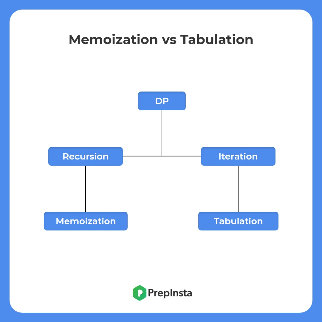
The Five Concepts for Today
- Top-Down with Memoization: Optimizing recursion by remembering results.
- Bottom-Up with Tabulation: Building an iterative solution from the ground up.
- Memoization vs. Tabulation: A detailed comparison of their trade-offs.
- Space Optimization: A key refinement for elite-level solutions.
- Applying the Strategies: Implementing both approaches for the Rod Cutting problem.
Concept 1: Top-Down with Memoization - "Remembering Your Work"
Technical Explanation
Memoization is the technique of optimizing a recursive algorithm by storing the results of expensive function calls and returning the cached result when the same inputs occur again. It's a top-down approach because you start with the main problem (e.g., fib(n)) and recursively break it down.
The process is a straightforward modification of the naive recursive solution we saw in the last lesson:
- Create a cache (an array or a hash map) to store computed results. Initialize it with a sentinel value (like -1 or
None) to indicate that a subproblem hasn't been solved yet. - In your recursive function, before any computation, check if the result for the current state is already in the cache.
- If it is (a "cache hit"), return the stored value immediately.
- If it isn't (a "cache miss"), compute the result recursively, store it in the cache, and then return it.
This process eliminates the redundant computations of overlapping subproblems, drastically improving the time complexity. For the Fibonacci sequence, this changes the complexity from exponential () to linear ().
Metaphor: The Caching Database Query
Think of memoization like a database query cache. A web application needs to fetch user profile data.
- Without Memoization (Naive Recursion): Every time any part of the app needs User #123's profile, it performs a full, expensive query on the main database.
- With Memoization: The first time the app needs User #123's profile, it queries the database and stores the result in a fast in-memory cache (like Redis). The next time any part of the app asks for the same profile, it pulls the data directly from the cache, bypassing the slow database entirely. The cache acts as our "memo."
Implementation: Memoized Fibonacci
Below is the Python code for a memoized Fibonacci function. Notice how it's just the naive recursive function with a memo dictionary added.
def fib_memo(n, memo={}):
    """
    Calculates the n-th Fibonacci number using top-down memoization.
    Time Complexity: O(n)
    Space Complexity: O(n) for the recursion stack and memo dictionary.
    """
    # If the result for n is already cached, return it.
    if n in memo:
        return memo[n]

    # Base cases for the recursion.
    if n <= 1:
        return n

    # Compute, cache, and return the result.
    result = fib_memo(n - 1, memo) + fib_memo(n - 2, memo)
    memo[n] = result

    return result

# Note: A new dictionary is created for each top-level call to avoid issues
# with Python's default mutable arguments.
print(f"fib_memo(50) = {fib_memo(50, {})}")
# This runs instantly, unlike the naive version.
Dynamic Programming - Top Down Memoization & Bottom Up Tabulation - DSA Course in Python Lecture 15
The following video by Greg Hogg provides a clear visualization and implementation of memoization. It shows how adding a cache prunes the recursion tree we saw in the last lesson.
Watch from 03:27 to 13:07. First, focus on the visualization (03:27-07:13) of the recursion tree to see the overlapping subproblems. Then, pay close attention to how the code is modified with a memo dictionary to avoid re-computation (07:13-13:07).
Concept 2: Bottom-Up with Tabulation - "Building From the Ground Up"
Technical Explanation
Tabulation is an iterative approach to DP. Instead of starting from the top n and going down, you start from the base cases and build your way up to the solution. You create a "table" (usually an array) and fill it sequentially.
The process for Fibonacci is as follows:
- Create a table
dpof sizen+1to store the Fibonacci numbers from 0 ton. - Initialize the base cases directly in the table:
dp[0] = 0anddp[1] = 1. - Iterate from
i = 2up ton. In each iteration, calculatedp[i]using the previously computed values in the table:dp[i] = dp[i-1] + dp[i-2]. - The final answer is the last value in the table,
dp[n].
This approach avoids recursion altogether, which can be a performance benefit by eliminating the overhead of function calls and the risk of stack overflow for very deep recursions.
Metaphor: The Skyscraper Construction
Building a skyscraper is a bottom-up process. You can't start by building the penthouse on the 100th floor.
- You lay the foundation (the base cases, F(0) and F(1)).
- You build the 1st floor, then the 2nd, then the 3rd, and so on. Each new floor relies on the structural integrity of the floors beneath it.
- The completed penthouse (the final solution, F(n)) is the last thing you build, resting upon the solutions to all the smaller subproblems (the lower floors).
The table in tabulation is your architectural blueprint and the building itself, growing floor by floor.
Implementation: Tabulated Fibonacci
def fib_tab(n):
    """
    Calculates the n-th Fibonacci number using bottom-up tabulation.
    Time Complexity: O(n)
    Space Complexity: O(n) for the dp table.
    """
    if n <= 1:
        return n

    # 1. Create a table of size n+1.
    dp = [0] * (n + 1)

    # 2. Initialize base cases.
    dp[1] = 1

    # 3. Iterate and fill the table.
    for i in range(2, n + 1):
        dp[i] = dp[i-1] + dp[i-2]

    # 4. The answer is in the last cell.
    return dp[n]

print(f"fib_tab(50) = {fib_tab(50)}")
Dynamic Programming - Top Down Memoization & Bottom Up Tabulation - DSA Course in Python Lecture 15
The same video from Greg Hogg continues by explaining the tabulation approach. It clearly connects the iterative logic to the sequence of Fibonacci numbers.
Now, watch from 13:07 to 18:27. Focus on how the dp array is created and filled iteratively. This demonstrates the bottom-up strategy in action.
Concept 3: Memoization vs. Tabulation - The Core Trade-offs
Choosing between memoization and tabulation is a key architectural decision in solving a DP problem. While both often have the same time complexity, their performance characteristics and ease of implementation can differ.
The article 'Tabulation vs Memoization' from GeeksforGeeks provides a concise comparison table that summarizes the key differences. This is an excellent reference for interviews.
Read the introductory section and focus on the comparison table. Pay special attention to the rows for 'Speed', 'Code', and 'Subproblem solving'.
Here is a summary of the trade-offs:
| Aspect | Memoization (Top-Down) | Tabulation (Bottom-Up) |
|---|---|---|
| Approach | Recursive. Starts from the main problem and breaks it down. | Iterative. Starts from the base cases and builds up. |
| Code Structure | Often more intuitive; a simple modification of a pure recursive solution. | Can require more thought to determine the correct iteration order and table structure. |
| Performance | Can be slower due to recursion overhead (function call stack management). | Generally faster in practice as iterative loops have less overhead than deep recursion. |
| Stack Overflow | Prone to stack overflow errors if the recursion depth is very large. | No risk of stack overflow, as it's iterative. |
| Subproblem Scope | Solves only the subproblems that are actually required to reach the solution. | Solves all subproblems up to n, even if some are not strictly necessary for the final result. |
| When to Prefer | When the state space is sparse and only a fraction of subproblems need solving. | When all or most subproblems must be solved. Also preferred for space optimization. |
Metaphor: Route Planning
Imagine finding the shortest driving time from San Francisco to New York.
- Memoization (Top-Down): You look at your map and see you need to get to NY. You decide your route will go through Chicago. Now you have a new subproblem: find the shortest time from SF to Chicago. You recursively break down the trip until you reach known, small segments. You only calculate routes you actually need.
- Tabulation (Bottom-Up): You get a giant chart and systematically calculate the shortest driving time between every pair of major cities in the US, starting with adjacent ones. By the time you're done, you have a lookup table for everything. To find the SF-to-NY time, you just look it up. It's more work up-front, but the table is complete.
Concept 4: Space Optimization - The Final Polish
For many DP problems, tabulation opens the door to a crucial final optimization: reducing space complexity.
Technical Explanation
Look at the tabulation code for fib_tab(n). To calculate dp[i], we only need dp[i-1] and dp[i-2]. We never need dp[i-3] or any earlier values again. This means we don't need to store the entire dp table of size . We only need to keep track of the two most recent values.
By using two variables (e.g., prev1 and prev2) instead of a full array, we can reduce the space complexity from to , while keeping the time complexity at . This is a massive improvement and is often expected in interviews at elite companies.
Metaphor: The Rolling Update
Think of calculating a running average of a stream of numbers. You don't need to store every number you've ever seen. You only need the current average and the total count. When a new number arrives, you use these two pieces of information to calculate the new average, then discard the old one. You are maintaining a constant amount of state, regardless of how long the stream is.
Implementation: Space-Optimized Fibonacci
def fib_optimized(n):
    """
    Calculates the n-th Fibonacci number using bottom-up tabulation
    with space optimization.
    Time Complexity: O(n)
    Space Complexity: O(1)
    """
    if n <= 1:
        return n

    # We only need the previous two values.
    prev2, prev1 = 0, 1

    # Iterate from 2 up to n.
    for _ in range(2, n + 1):
        # Calculate the current value.
        current = prev1 + prev2

        # Update the pointers for the next iteration.
        prev2 = prev1
        prev1 = current

    return prev1

print(f"fib_optimized(50) = {fib_optimized(50)}")
Dynamic Programming - Top Down Memoization & Bottom Up Tabulation - DSA Course in Python Lecture 15
The Greg Hogg video concludes by showing this exact space optimization. This is the final step in refining a DP solution.
Watch the final segment from 18:27 to 20:08. See how the array is replaced by two variables, reducing space to O(1).
Concept 5: Applying the Strategies - The Rod Cutting Problem
Let's apply these techniques to a different, more complex problem to see how the patterns generalize.
Problem: Given a rod of length n and a prices array where prices[i] is the price of a piece of length i+1, find the maximum value obtainable by cutting up the rod and selling the pieces.
Example: prices = [1, 5, 8, 9]. For a rod of length n=4, we could cut it into two pieces of length 2 (price 5+5=10), or four pieces of length 1 (price 1+1+1+1=4), or one piece of length 1 and one of length 3 (price 1+8=9), etc. The optimal is to cut it into two pieces of length 2, for a total value of 10.
The complexity here will be because for each length i from 1 to n, we consider all possible cuts j from 1 to i.
The GeeksforGeeks article we referenced earlier provides full Python implementations for both memoization and tabulation for the Rod Cutting problem. Study these to see the patterns on a new problem.
In the article, find the 'Rod Cutting Problem' section. Examine the Python code for both 'Top-Down DP (Memoization)' and 'Bottom-Up DP (Tabulation)'. Compare their structures to the Fibonacci examples.
Implementation: Memoized Rod Cutting
def rod_cut_memo(prices, n, memo):
    """
    Solves the Rod Cutting problem with memoization.
    Time Complexity: O(n^2)
    Space Complexity: O(n)
    """
    if n in memo:
        return memo[n]
    if n <= 0:
        return 0

    max_val = 0
    # Try every possible first cut.
    for i in range(n):
        # prices[i] is for a piece of length i+1.
        # The remaining rod length is n - (i+1).
        current_val = prices[i] + rod_cut_memo(prices, n - (i + 1), memo)
        if current_val > max_val:
            max_val = current_val

    memo[n] = max_val
    return max_val

prices = [1, 5, 8, 9, 10, 17, 17, 20]
n = len(prices)
print(f"Max profit (Memoization) for rod of length {n}: {rod_cut_memo(prices, n, {})}")
Implementation: Tabulated Rod Cutting
def rod_cut_tab(prices, n):
    """
    Solves the Rod Cutting problem with tabulation.
    Time Complexity: O(n^2)
    Space Complexity: O(n)
    """
    # dp[i] will store the max profit for a rod of length i.
    dp = [0] * (n + 1)

    # Build the table dp[] in bottom-up manner.
    for i in range(1, n + 1):
        max_val = 0
        for j in range(i):
            # Cut a piece of length j+1, price prices[j].
            # Remaining length is i - (j+1). Max profit for that is dp[i-(j+1)].
            max_val = max(max_val, prices[j] + dp[i - (j + 1)])
        dp[i] = max_val

    return dp[n]

prices = [1, 5, 8, 9, 10, 17, 17, 20]
n = len(prices)
print(f"Max profit (Tabulation) for rod of length {n}: {rod_cut_tab(prices, n)}")
Test your understanding!
The "Climbing Stairs" problem is another DP classic: You are climbing a staircase. It takes n steps to reach the top. Each time you can either climb 1 or 2 steps. In how many distinct ways can you climb to the top?
The naive recursive solution is ways(n) = ways(n-1) + ways(n-2).
Your task: Write a space-optimized, bottom-up (tabulation) function to solve this. What are its time and space complexities?
Show answer
This problem has the exact same recurrence relation as Fibonacci. Therefore, we can use the same space-optimized approach.
def climb_stairs(n):
    """
    Calculates the number of ways to climb n stairs with space optimization.
    Time Complexity: O(n)
    Space Complexity: O(1)
    """
    if n <= 2:
        return n

    # prev2 stores ways(i-2), prev1 stores ways(i-1)
    prev2, prev1 = 1, 2

    for i in range(3, n + 1):
        current = prev1 + prev2
        prev2 = prev1
        prev1 = current

    return prev1

print(f"Ways to climb 10 stairs: {climb_stairs(10)}") # Expected: 89
The time complexity is because of the single loop up to n. The space complexity is because we only use a few variables to store the state, regardless of the value of n.
Conclusion
Today you've moved from theory to practice, implementing the two core DP strategies. This is a massive step toward mastering DP for interviews and real-world problem-solving.
Key Takeaways:
- Memoization (Top-Down): A natural extension of recursion. Easy to write and only solves necessary subproblems, but carries recursion overhead.
- Tabulation (Bottom-Up): An iterative approach that is often faster and safer from stack overflows. It builds a solution from base cases upwards.
- Trade-offs are Key: Tabulation is generally preferred for its performance and because it enables space optimization.
- Space Optimization: Always look for opportunities to reduce the space of your tabulation solution. If
dp[i]only depends ondp[i-1]anddp[i-2], you can likely achieve space. - Patterns Generalize: The memoization and tabulation patterns you learned with Fibonacci are directly applicable to more complex problems like Rod Cutting.
Preview of the Next Lesson:
With these foundational implementation skills, we are ready to tackle more complex DP problems. In the next lesson, we will dive into 1D and 2D DP problems. You'll solve classics like Longest Common Subsequence and Edit Distance, learning how to define a 2D state and build a 2D DP table.