Analyzing Recursive Algorithms with Recurrence Relations

Concept 1: From Recursive Code to Recurrence Relations

The first step in analyzing any recursive algorithm is to translate its structure into a mathematical formula. This formula is called a recurrence relation.

Technical Explanation

A recurrence relation defines a function in terms of itself, just like a recursive algorithm calls itself. It consists of two parts:

1. Base Case(s): The cost of solving the smallest possible problem (e.g., an array of size 1), which doesn't lead to further recursion. We usually express this as a constant, like $T(1)=c$ or simply $T(1)=\Theta (1)$.
2. Recursive Case: An equation that expresses the cost for an input of size $n$, $T(n)$, in terms of the cost of solving smaller subproblems.

Let's model the two key recursive algorithms from our last lesson:

• Binary Search: In each step, it performs one comparison ($\Theta (1)$ work) and then makes one recursive call on a subproblem of half the size ($n/2$).

  • Recurrence Relation: $T(n)=T(n/2)+\Theta (1)$

• Merge Sort: In each step, it makes two recursive calls on subproblems of half the size ($n/2$) and then combines the results by merging the two sorted halves, which takes linear time ($\Theta (n)$ work).

  • Recurrence Relation: $T(n)=2T(n/2)+\Theta (n)$

Metaphor: A Self-Referencing Recipe

Think of a recurrence relation as a recipe for a fractal-like dish.

• Recursive Case: "To cook a 'Mega-Meal' for n people, first prepare two 'Half-Meals' (for n/2 people each), and then spend n minutes combining them." This corresponds to $T(n)=2T(n/2)+n$.
• Base Case: "A 'Single-Serving' meal takes 1 minute to prepare." This corresponds to $T(1)=1$.
  Our goal is to solve this "recipe" to find the total cooking time for the Mega-Meal.

Interview Question

"Consider the following Python function that calculates the nth Fibonacci number. Write down the recurrence relation for its time complexity. Don't solve it yet, just model it."

def fib(n):
    if n <= 1:
        return n
    return fib(n-1) + fib(n-2)

Answer: "The base cases n <= 1 take constant time, so $T(0)=T(1)=\Theta (1)$. The recursive step makes two calls, one to fib(n-1) and another to fib(n-2), and then does a constant amount of work (one addition). Therefore, the recurrence relation is $T(n)=T(n-1)+T(n-2)+\Theta (1)$."

Concept 2: The Recursion Tree Method — Visualizing the Cost

The recursion tree method is a powerful way to visualize the work done by a recursive algorithm and make an educated guess about its complexity. It's often the most intuitive first step.

Technical Explanation

In this method, we draw a tree to represent the recursive calls. Each node in the tree represents the cost of a single subproblem, and the total cost of the algorithm is the sum of costs of all nodes.

Let's analyze the Merge Sort recurrence: $T(n)=2T(n/2)+n$.

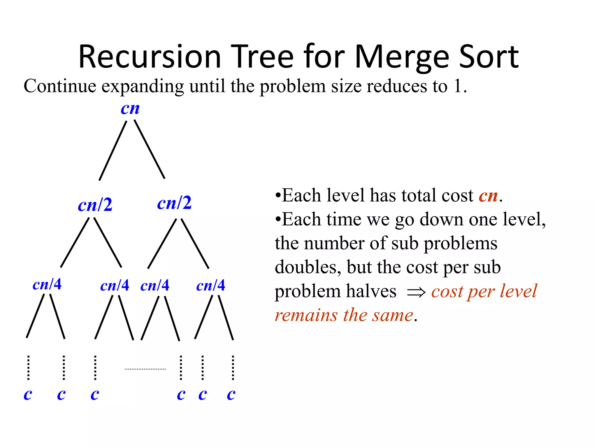
Here’s how to break it down:

1. Root: The root of the tree represents the initial call. The work done at this top level (the cost of the final merge) is $n$. This call spawns two children for the subproblems.
2. Level 1: We have two subproblems of size $n/2$. The work for each is $n/2$. The total work at this level is $2\times (n/2)=n$.
3. Level i: At depth i, we have $2^i$ subproblems, each of size $n/2^i$. The work for each is $n/2^i$. The total work at this level is $2^i\times (n/2^i)=n$.
4. Tree Depth: The recursion stops when the subproblem size is 1. This happens when $n/2^k=1$, which solves to $k={\log }_{2}n$. So, the tree has ${\log }_{2}n$ levels.
5. Total Cost: Since each of the $\log n$ levels contributes $n$ to the total work, the overall time complexity is $\text{levels}\times \text{work per level}=(\log n)\times n=\Theta (n\log n)$.

This method gives us a strong hypothesis for the algorithm's complexity.

Metaphor: A Project Delegation Hierarchy

Imagine a CEO (the root call) needs to complete a project.

• She spends n hours on high-level strategy (the work at the root).
• She delegates the project to two VPs (2 children). Each VP works on a project of half the scope (n/2 hours of work) and delegates to two directors.
• The total work at the VP level is $2\times (n/2)=n$ hours.
• This continues down the hierarchy. If the work at every level of the company hierarchy sums to n hours, and the hierarchy is $\log n$ levels deep, the total project cost is $n\log n$ person-hours.

Concept 3: The Substitution Method — Proving the Guess

The recursion tree gives us a good guess, but it's not a formal proof. The substitution method uses mathematical induction to rigorously prove that our guess is correct.

Technical Explanation

The process has two main steps:

1. Guess the solution: We use the recursion tree or intuition to guess a bound (e.g., $T(n)\le cn\log n$).
2. Prove by induction:
   • Inductive Hypothesis: Assume the guess is true for all integers smaller than $n$.
   • Inductive Step: Use the recurrence relation and the hypothesis to prove that the guess is also true for $n$.

Let's prove that $T(n)=2T(n/2)+n$ is $O(n\log n)$.

1. Guess: From our recursion tree, we guess $T(n)=O(n\log n)$. Formally, we want to prove $T(n)\le cn\log n$ for some constant $c>0$ and for all $n\ge n_0$.
2. Inductive Hypothesis: Assume $T(k)\le ck\log k$ for all $k<n$. This implies it holds for $k=n/2$, so $T(n/2)\le c(n/2)\log (n/2)$.
3. Inductive Step: Substitute this into the recurrence: $$\begin{array}{rlr}T(n)& =2T(n/2)+n& \\ & \le 2\left(c\frac{n}{2}\log \left(\frac{n}{2}\right)\right)+n& \text{(Substitute hypothesis)}\\ & =cn\left(\log n-\log 2\right)+n& \text{(Logarithm properties)}\\ & =cn\log n-cn{\log }_{2}2+n& \text{(Assuming base 2 log)}\\ & =cn\log n-cn+n& \end{array}$$ We need to show this is $\le cn\log n$. This holds if $cn\log n-cn+n\le cn\log n$, which simplifies to $-cn+n\le 0$, or $n\le cn$. This is true for any $c\ge 1$. We have successfully proved our guess.

Interview Question

"Suppose you're analyzing a recurrence and use the substitution method. You guess the bound is $T(n)\le cn$ and your inductive step results in $T(n)\le cn+d$, where $d$ is a positive constant. Have you proven your guess? If not, what does this result suggest?"

Answer: "No, the guess has not been proven. The substitution method requires proving the exact form of the inductive hypothesis. Deriving $T(n)\le cn+d$ fails to prove $T(n)\le cn$. This result suggests that the guess is too low. The extra term, which might seem small, will accumulate at each level of recursion, indicating that the true complexity is likely a higher order than $O(n)$."

Concept 4: The Master Theorem — The Ultimate Shortcut

For a large class of divide-and-conquer algorithms, we can bypass the recursion tree and substitution methods and get an answer directly using a powerful formula known as the Master Theorem.

Technical Explanation

The Master Theorem applies to recurrences of the form:
$T(n)=aT(n/b)+f(n)$
where:

• $a\ge 1$ is the number of subproblems.
• $b>1$ is the factor by which the input size is reduced.
• $f(n)$ is the cost of the work done outside the recursive calls (dividing the problem and combining the results).

The theorem compares the function $f(n)$ to $n^{{\log }_{b}a}$. This critical value represents the rate of growth of the work done at the leaves of the recursion tree. The intuition is to see which part of the algorithm dominates: the work at the root ($f(n)$) or the work at the leaves ($n^{{\log }_{b}a}$).

There are three cases:

1. Case 1: Root-dominated. If $f(n)=O(n^{{\log }_{b}a-ϵ})$ for some constant $ϵ>0$. (i.e., $f(n)$ grows polynomially slower than $n^{{\log }_{b}a}$).

   • Solution: $T(n)=\Theta (n^{{\log }_{b}a})$

2. Case 2: Balanced. If $f(n)=\Theta (n^{{\log }_{b}a})$. (i.e., $f(n)$ grows at the same rate as $n^{{\log }_{b}a}$).

   • Solution: $T(n)=\Theta (n^{{\log }_{b}a}\log n)$

3. Case 3: Leaf-dominated. If $f(n)=\Omega (n^{{\log }_{b}a+ϵ})$ for some constant $ϵ>0$, AND if $af(n/b)\le cf(n)$ for some constant $c<1$ and sufficiently large $n$ (this is a "regularity condition").

   • Solution: $T(n)=\Theta (f(n))$

Applying the Master Theorem:

• Merge Sort: $T(n)=2T(n/2)+n$

  • $a=2,b=2,f(n)=n$.
  • Critical value: $n^{{\log }_{2}2}=n^1=n$.
  • $f(n)=\Theta (n)$, which matches the critical value. This is Case 2.
  • Solution: $T(n)=\Theta (n\log n)$.

• Binary Search: $T(n)=T(n/2)+1$

  • $a=1,b=2,f(n)=1$.
  • Critical value: $n^{{\log }_{2}1}=n^0=1$.
  • $f(n)=\Theta (1)$, which matches. This is Case 2.
  • Solution: $T(n)=\Theta (1\cdot \log n)=\Theta (\log n)$.

• Example from Concept 2: $T(n)=3T(n/4)+n^2$

  • $a=3,b=4,f(n)=n^2$.
  • Critical value: $n^{{\log }_{4}3}\approx n^{0.79}$.
  • $f(n)=n^2$ grows polynomially faster than $n^{0.79}$. This is Case 3. We check the regularity condition: $3(n/4{)}^2=(3/16)n^2\le (3/16)n^2$. This holds for $c=3/16<1$.
  • Solution: $T(n)=\Theta (n^2)$.

Concept 5: Advanced Recurrences & Method Choice

Not all recurrences fit the Master Theorem's tidy format. For these, we must rely on more fundamental methods or transformations.

Technical Explanation

Consider the recurrence for an algorithm that works on a data structure like a B-tree or performs a search on a range by taking its square root:
$T(n)=2T(\sqrt{n})+\log n$
This recurrence is not in the form $T(n)=aT(n/b)+f(n)$, so the Master Theorem does not apply. Here we can use a change of variables (a domain transformation) to convert it into a familiar form.

1. Define a new variable: Let $m={\log }_{2}n$. This implies $n=2^m$.
2. Substitute into the recurrence:
   • The term $T(n)$ becomes $T(2^m)$.
   • The term $T(\sqrt{n})$ becomes $T((2^m{)}^{1/2})=T(2^{m/2})$.
   • The term $\log n$ becomes $m$.
     The recurrence is now: $T(2^m)=2T(2^{m/2})+m$.
3. Define a new function: Let $S(m)=T(2^m)$. Our recurrence transforms to:
   $S(m)=2S(m/2)+m$
   This is the exact recurrence for Merge Sort! We already know its solution is $S(m)=\Theta (m\log m)$.
4. Convert back: Now we substitute back our original variables. Since $S(m)=T(n)$ and $m=\log n$:
   $T(n)=\Theta (\log n\cdot \log (\log n))$
   This technique demonstrates the power of transforming a problem into one you've already solved.

Choosing Your Method:

• Recursion Tree: Always a great starting point for building intuition and generating a guess. It's visual and hard to get wrong conceptually.
• Master Theorem: Your first choice for any divide-and-conquer recurrence that fits the $aT(n/b)+f(n)$ pattern. It's the fastest method.
• Substitution Method: The fundamental proof technique. Use it when the Master Theorem doesn't apply, or when an interviewer explicitly asks you to "prove from first principles."
• Transformations: A powerful tool for recurrences with unusual arguments (like $\sqrt{n}$ or $n-k$). The goal is to transform them into a form solvable by the other methods.

Conclusion

Today, you've acquired the essential mathematical toolkit for analyzing recursive algorithms. You can now formally justify the performance claims we've made in previous lessons.

Key Takeaways:

• Recurrence Relations are the mathematical models of recursive algorithms.
• The Recursion Tree Method provides a visual way to sum up the work done at all levels of recursion and generate a complexity guess.
• The Substitution Method uses mathematical induction to formally prove a complexity bound, making it the most rigorous technique.
• The Master Theorem is a powerful shortcut for solving a common class of divide-and-conquer recurrences by comparing the work at the root versus the leaves.
• For non-standard recurrences, techniques like change of variables can transform them into a solvable form.

Preview of the Next Lesson

We've now completed our initial deep dive into complexity analysis. Our next lesson will transition from theory to practice by starting our exploration of core sorting algorithms. We'll begin with the simpler, $O(n^2)$ algorithms: Bubble Sort, Insertion Sort, and Selection Sort. While not optimal, analyzing their mechanisms provides a crucial foundation for understanding the more advanced $O(n\log n)$ algorithms to come.