Welcome to your third lesson in our "Algorithmic Foundations and Complexity" module. In our previous lessons, we established how to analyze an algorithm's efficiency using Big O for time complexity and also dissected its memory usage via space complexity. We've heavily focused on the idea of an upper bound, or a "performance guarantee."
Today, we'll add crucial nuance to that analysis. An algorithm's performance isn't a single, static number; it often changes dramatically based on the nature of the input. This lesson fulfills the learning outcome: Explain best, average, and worst-case complexity scenarios with concrete examples. By the end, you will be able to distinguish between these scenarios, apply the correct notation for each, and understand how these differences drive real-world engineering decisions.
Concept 1: The Three Faces of Performance: Best, Average, and Worst Case
So far, when we've said an algorithm is , we've implicitly been talking about its worst-case behavior. However, to get a complete picture, we need to consider the full spectrum of its performance.
Technical Explanation
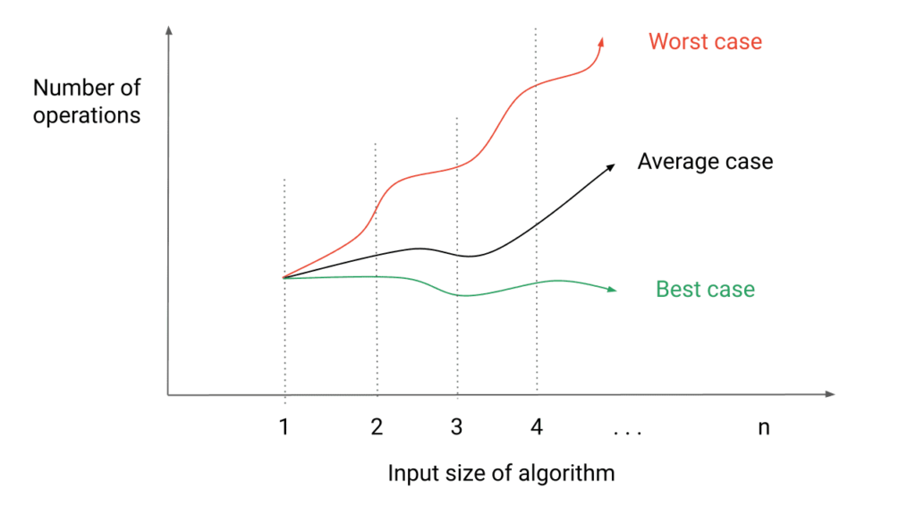
For a given algorithm and an input of size , we analyze its performance under three different conditions:
- Best Case: This scenario represents the most favorable input, leading to the minimum number of operations. It's the "lucky shot" where the algorithm finishes as quickly as possible.
- Worst Case: This is the scenario we've focused on. It represents the least favorable input, causing the algorithm to perform the maximum number of operations. It provides a crucial guarantee: the algorithm will never perform worse than this.
- Average Case: This describes the expected performance of an algorithm averaged over all possible inputs of size . This is often the most practical measure of real-world performance but can be the most mathematically challenging to calculate precisely.
Metaphor: Finding a Book in a Library
Imagine you're looking for a specific book on a single, long shelf containing n books.
- Best Case: The book you want is the very first one you check. You're done instantly.
- Worst Case: The book is the very last one on the shelf. You have to scan through all
nbooks to find it. - Average Case: Assuming the book could be anywhere with equal probability, you'd expect to check about half the books,
n/2, on average.
Example: Linear Search
Let's apply this to the simple algorithm of linear search, which iterates through an array to find a target value.
def linear_search(arr, target):
    """
    Searches for a target in an array by checking each element sequentially.
    Let n = len(arr).
    """
    for i in range(len(arr)):
        if arr[i] == target:
            return i  # Found it!
    return -1 # Not in the array

# Best Case: target is arr[0]. 1 comparison.
# Worst Case: target is arr[n-1] or not in the array. n comparisons.
# Average Case: On average, we check n/2 elements.
Best Case, Worst Case and Average Case Analysis of an Algorithm (With Notes)
To see a detailed walkthrough of these concepts, watch the following video. It uses the linear search example to clearly explain what best, worst, and average cases mean.
Watch from the beginning to 08:40. The video introduces the three cases with a simple analogy and then applies them directly to a linear search algorithm, analyzing the number of comparisons for each scenario.
Interview Question
"In system design and performance analysis, why is worst-case complexity (Big O) often prioritized over best-case or even average-case?"
Answer: "Worst-case complexity provides a performance guarantee. For critical systems, especially those with Service Level Agreements (SLAs), we need to know the absolute upper limit on response time or resource consumption. Relying on the average or best case is optimistic and can lead to system failure under specific, but possible, 'unlucky' loads. The worst case gives us a solid baseline for capacity planning and ensuring reliability."
Concept 2: The Notational Zoo: Big O, Omega (Ω), and Theta (Θ)
To discuss these different cases with precision, computer scientists use specific notations for each type of bound.
Technical Explanation
- Big O (O): Upper Bound. Used for the worst-case. An algorithm with runtime is if its runtime is at most a constant multiple of for large . It gives a ceiling on performance.
- Big Omega (Ω): Lower Bound. Used for the best-case. An algorithm is if its runtime is at least a constant multiple of for large . It provides a performance floor.
- Big Theta (Θ): Tight Bound. Used when the best and worst cases belong to the same complexity class. An algorithm is if its runtime is both and . It "sandwiches" the function, describing its growth rate precisely.
For linear search:
- The best case is .
- The worst case is .
- Since the best and worst cases differ (), we cannot describe the algorithm with a single notation.
For an algorithm that always finds the maximum element in an array by iterating through it once:
- The best case is (you must look at every element).
- The worst case is .
- Since the best and worst cases are the same, we can say the algorithm is .
Asymptotic Notations 101: Big O, Big Omega, & Theta (Asymptotic Analysis Bootcamp)
The following video gives a mathematically rigorous yet intuitive graphical explanation of these three notations. It's essential for truly understanding the difference between an upper, lower, and tight bound.
Watch from 16:01 to 21:21. The presenter clearly visualizes how Big Omega provides a 'floor' for a function, Big O provides a 'ceiling', and Big Theta 'sandwiches' it, combining both.
Metaphor: Estimating Project Time
You're a software engineering manager estimating a project.
- Big Omega (Ω): "This project will take at least 2 weeks." (Lower bound, best-case scenario).
- Big O (O): "This project will take at most 6 weeks." (Upper bound, worst-case scenario, accounting for risks).
- Big Theta (Θ): "This project is a standard CRUD app; it will take around 3 weeks." (Tight bound, because the best and worst cases are very similar).
Interview Question
"Is it correct to say an algorithm with a Θ(n) runtime is also O(n^2)? Why or why not?"
Answer: "Yes, that is technically correct, though not very useful. Big O provides an upper bound. If an algorithm's runtime is tightly bound by (i.e., ), then its runtime is also guaranteed to be less than . So, is a valid, but loose, upper bound. The tightest possible bound, , is always the most descriptive and what's expected in an interview."
Concept 3: Case Analysis in Action: Linear vs. Binary Search
Let's analyze two different algorithms for the same problem—searching—to see how their performance cases differ. This highlights how algorithm choice is driven by both performance and input preconditions.
Technical Explanation
We will compare linear search on an unsorted array with binary search on a sorted array.
| Algorithm | Best Case | Average Case | Worst Case | Precondition |
|---|---|---|---|---|
| Linear Search | (target is first) | (target is last/absent) | None | |
| Binary Search | (target is middle) | Array must be sorted |
Binary search's logarithmic complexity stems from its "divide and conquer" strategy. With each comparison, it eliminates half of the remaining search space.
Metaphor: The Dictionary
- Linear Search: You're looking for the word "Zebra" in a dictionary but you don't know it's alphabetized. You start at "Aardvark" and read every single entry until you find it.
- Binary Search: You know the dictionary is alphabetized. You open it to the middle (say, the 'M' section). You see 'Z' comes after 'M', so you ignore the entire first half and repeat the process on the second half. This is exponentially faster.
Python Code Implementations
# Binary Search (Iterative)
def binary_search(sorted_arr, target):
    """
    Searches for a target in a sorted array using the divide and conquer method.
    Let n = len(sorted_arr).
    """
    low = 0
    high = len(sorted_arr) - 1

    while low <= high:
        mid = (low + high) // 2  # Find the middle index

        # Best Case: target is at mid on the first try. O(1)
        if sorted_arr[mid] == target:
            return mid
        elif sorted_arr[mid] < target:
            low = mid + 1  # Target is in the right half
        else:
            high = mid - 1 # Target is in the left half

    return -1 # Target not found

# The number of iterations is the number of times we can halve n, which is log_2(n).
# So, the worst and average cases are O(log n).
Design Trade-offs & Real-World Application
Binary search is vastly superior in performance, but it comes with a critical precondition: the data must be sorted.
- Scenario 1: Write-heavy, infrequent reads. If you have a system where data is constantly being added (like logging), but searches are rare, the cost of keeping the data sorted outweighs the benefit of fast searches. A linear scan might be acceptable.
- Scenario 2: Read-heavy, infrequent writes. If you have a dataset that rarely changes but is searched millions of time per second (like a product catalog on an e-commerce site), the one-time cost of sorting () is easily paid back by the incredibly fast searches. This is why database indexes are structured like trees, which enable binary-search-like operations.
Concept 4: Deeper Dive: Sorting and "Adaptive" Algorithms
The characteristics of an input can have a profound impact on sorting algorithms. An algorithm that performs well on nearly-sorted data is called adaptive. Insertion Sort is a classic example.
Technical Explanation
Insertion Sort works by building a sorted subarray at the beginning of the list. It takes each unsorted element and "inserts" it into its correct spot in the sorted part.
- Best Case:
When the array is already sorted. The outer loop runsntimes, but the inner loop to find the insertion point immediately finds that the element is already in the correct place, making just one comparison. - Worst Case:
When the array is reverse-sorted. For each element, it must be compared against and shifted past every other element in the sorted subarray. - Average Case:
For a randomly shuffled array, on average, each element must be shifted past half of the elements in the sorted subarray.
Metaphor: Arranging a Hand of Playing Cards
When you're dealt cards, you typically pick them up one by one and insert them into the correct sorted position in your hand.
- Best Case: The dealer hands you the cards already in perfect order (e.g., 2, 3, 4, 5...). You just verify each card's position with a single glance. Fast.
- Worst Case: The dealer hands them to you in reverse order (e.g., King, Queen, Jack...). For each new card, you have to shift your entire hand to make room at the beginning. Slow.
Python Code: Insertion Sort
def insertion_sort(arr):
    """Sorts an array using the insertion sort algorithm."""
    # Start from the second element (the first is a sorted subarray of size 1)
    for i in range(1, len(arr)):
        key = arr[i]
        j = i - 1

        # In the best case (sorted array), this `while` condition is
        # immediately false. The inner loop never runs. Total time = O(n).

        # In the worst case (reverse-sorted array), this loop runs i times
        # for each element. This leads to 1+2+3...+(n-1) = n*(n-1)/2 ops, so O(n^2).
        while j >= 0 and key < arr[j]:
            arr[j + 1] = arr[j]
            j -= 1
        arr[j + 1] = key
    return arr
Real-World Application: Timsort
Python's built-in sort() and sorted() functions use an algorithm called Timsort. Timsort is a hybrid algorithm that is optimized for real-world data, which is often partially sorted. It identifies sorted "runs" in the data and uses Insertion Sort to merge these small runs, leveraging its performance on nearly-sorted data. For larger runs, it switches to Merge Sort. This adaptiveness makes it extremely efficient in practice.
Concept 5: The Pivotal Role of Average Case: Quicksort
Quicksort is one of the most widely used sorting algorithms, a fact that might seem surprising given its worst-case performance. This is the ultimate example of how a superior average-case performance can dominate practical decision-making.
Technical Explanation
Quicksort is another divide-and-conquer algorithm. It selects a 'pivot' element and partitions the array into two subarrays: elements less than the pivot and elements greater than the pivot. It then recursively sorts the subarrays.
- Worst Case:
This happens when the pivot selection is consistently poor. If the pivot is always the smallest or largest element, the partition will be extremely unbalanced (one subarray of size 0 and one of size ). This degrades the algorithm into something like a slow selection sort. This can easily happen if you always pick the first element as the pivot and the input array is already sorted. - Best Case:
This happens when the pivot is always the median element, perfectly splitting the array into two equal halves at each step. - Average Case:
This is the magic of Quicksort. If you choose the pivot randomly, the probability of repeatedly picking a bad pivot is astronomically low. On average, the partitions will be reasonably balanced, leading to the desired performance.
Metaphor: Delegating a Task
You need to sort a pile of n exam papers by score.
- Worst Case: You pick a pivot paper (e.g., score 99/100). You tell your team: "Alice, you sort the papers with scores less than 99. Bob, you sort the ones with scores greater than 99." Alice gets almost all the papers, and Bob gets none. You haven't effectively divided the work.
- Average Case (with random pivot): You pick a paper from the middle of the pile at random (e.g., score 75/100). You delegate the work. It's likely that Alice and Bob will get roughly equal-sized piles to work on. They can then repeat this process with their own teams. The work is divided efficiently at each step.
Why Quicksort is used in practice (over Merge Sort):
While Merge Sort has a guaranteed worst-case, Quicksort is often faster in practice.
- Lower Constant Factors: The inner loop of Quicksort involves simple swaps and comparisons, which are very fast on modern CPU architectures.
- Space Complexity: A standard Quicksort implementation is in-place, meaning it has an auxiliary space complexity of due to recursion depth on the stack. Merge Sort, by contrast, requires auxiliary space to create temporary arrays for merging, which is a significant disadvantage for large datasets.
Modern standard library implementations of Quicksort use clever pivot-selection strategies (like 'median-of-three') and switch to other algorithms like Heapsort if the recursion gets too deep, effectively eliminating the worst case in all but the most adversarial scenarios.
Interview Question
"Given that Quicksort has a dreaded O(n^2) worst case, why is it the default sorting algorithm in so many programming environments instead of Merge Sort or Heapsort, which guarantee O(n log n)?"
Answer: "The decision comes down to a trade-off between worst-case guarantees and practical, average-case performance. While Quicksort's worst case is poor, modern implementations use pivot strategies like random selection or median-of-three that make hitting the worst case statistically negligible. In its average case, which is overwhelmingly the norm, Quicksort is faster than Merge Sort and Heapsort due to lower constant factors in its operations and better cache locality. Furthermore, its in-place nature, requiring only auxiliary space compared to Merge Sort's , makes it far more memory-efficient for large datasets, which is often a decisive factor."
Conclusion
You have now completed your foundational tour of algorithmic complexity. You've moved beyond a one-dimensional view of performance to a more sophisticated, multi-faceted understanding.
Key Takeaways:
- An algorithm's performance is not fixed; it varies based on the input, which we categorize into best, average, and worst-case scenarios.
- We use specific notations for each bound: Big (Omega) for the best-case lower bound, Big O for the worst-case upper bound, and Big (Theta) for a tight bound when best and worst cases match.
- Algorithm choice involves trade-offs. The "best" algorithm depends on the data's characteristics (e.g., Insertion Sort is great for nearly-sorted data).
- In large-scale systems, an algorithm's average-case performance (like Quicksort's) is often more important than its theoretical worst-case, especially when the worst case can be mitigated with smart implementation (e.g., random pivots).
Preview of the Next Lesson
In this lesson, we analyzed recursive algorithms like Binary Search and Quicksort by stating their complexity. In the next lesson, we will learn the formal mathematical technique to derive these complexities. We will dive into mathematical recurrence relations, which allow you to precisely model the runtime of a recursive algorithm and solve for its Big O complexity.