Sorting Algorithms: O(n^2) and O(n log n)

Concept 1: The O(n²) Baseline — Bubble Sort

We'll start with the O(n²) family of algorithms. These are generally too slow for large datasets but are excellent for building foundational knowledge. Bubble Sort is the most classic example.

Technical Explanation

Bubble Sort works by repeatedly stepping through the list, comparing each pair of adjacent items, and swapping them if they are in the wrong order. After the first pass, the largest element will have "bubbled up" to its correct final position at the end of the list. Each subsequent pass bubbles up the next largest element, and this continues until the list is sorted. The algorithm can be optimized to terminate early if a pass is completed with no swaps, meaning the list is already sorted.

The time complexity arises from the nested loops. The outer loop runs n times, and the inner loop runs roughly n times for each outer iteration, leading to approximately $n\times n$ comparisons.

Metaphor: Lining Up by Height

Imagine a line of people of different heights who need to line up from shortest to tallest. With Bubble Sort, you'd tell the first person to compare their height with the person behind them. If they are taller, they swap places. Then, the (now potentially new) second person compares with the third, and so on. This process repeats down the line. After one full pass, the tallest person is guaranteed to be at the end. You then repeat the entire process, ignoring the last (now sorted) person, until everyone is in order.

Python Implementation

def bubble_sort(arr):
    n = len(arr)
    for i in range(n):
        # A flag to optimize and exit early if the list is already sorted
        swapped = False
        # The last i elements are already in place, so we don't need to check them
        for j in range(0, n - i - 1):
            # Traverse the array from 0 to n-i-1
            # Swap if the element found is greater than the next element
            if arr[j] > arr[j + 1]:
                arr[j], arr[j + 1] = arr[j + 1], arr[j]
                swapped = True
        if not swapped:
            break
    return arr

# Example
my_array = [64, 34, 25, 12, 22, 11, 90]
print(f"Sorted array: {bubble_sort(my_array)}")
# Output: Sorted array: [11, 12, 22, 25, 34, 64, 90]

Analysis & Trade-offs

• Time Complexity:
  • Worst-Case: $O(n^2)$ — When the array is in reverse order.
  • Average-Case: $O(n^2)$
  • Best-Case: $O(n)$ — When the array is already sorted and we use the swapped flag. The algorithm makes one pass and exits.
• Space Complexity: $O(1)$ — It's an in-place algorithm, meaning it sorts the array without requiring significant extra memory.
• Stability: Bubble Sort is a stable sort. This means that if two elements have equal values, their relative order in the original array will be preserved in the sorted array.

Interview Question

"Given its $O(n^2)$ complexity, is there ever a real-world scenario where you would consider using Bubble Sort?"

Answer: "In practice, almost never. Its performance is poor for any non-trivial dataset. Its main value is educational, as it's simple to understand and implement. For any production system, even Insertion Sort is a better choice for small datasets, and Merge Sort or Quick Sort are vastly superior for larger ones."

Concept 2: Building a Sorted Hand — Insertion Sort

Insertion Sort is another simple $O(n^2)$ algorithm that is often more efficient in practice than Bubble Sort.

Technical Explanation

Insertion Sort builds the final sorted array one item at a time. It iterates through the input elements and, for each element, it "inserts" it into its correct position within the already-sorted part of the array. To do this, it shifts all larger elements in the sorted part one position to the right.

Metaphor: Sorting a Hand of Cards

This is the classic analogy. Imagine you're dealt cards one by one. You pick up the first card and hold it. When you get the second card, you place it either before or after the first card. When the third card comes, you find its correct spot among the first two and insert it, shifting the others if needed. You repeat this for every card, always maintaining a sorted hand.

Python Implementation

def insertion_sort(arr):
    # Traverse through 1 to len(arr)
    for i in range(1, len(arr)):
        key = arr[i] # The card we're trying to place
        
        # Move elements of arr[0..i-1], that are greater than key,
        # to one position ahead of their current position
        j = i - 1
        while j >= 0 and key < arr[j]:
            arr[j + 1] = arr[j]
            j -= 1
        arr[j + 1] = key # Place the card in its correct spot
    return arr

# Example
my_array = [64, 34, 25, 12, 22, 11, 90]
print(f"Sorted array: {insertion_sort(my_array)}")
# Output: Sorted array: [11, 12, 22, 25, 34, 64, 90]

Analysis & Trade-offs

• Time Complexity:
  • Worst-Case: $O(n^2)$ — When the array is in reverse order.
  • Average-Case: $O(n^2)$
  • Best-Case: $O(n)$ — When the array is already sorted. The inner while loop condition is never met.
• Space Complexity: $O(1)$ — It's also an in-place algorithm.
• Stability: Yes, Insertion Sort is stable.
• Key Advantage: It's very efficient for small datasets and for datasets that are already "almost sorted." This property makes it a key component in more advanced hybrid algorithms like Timsort (Python's default sorting algorithm).

Interview Question

"You are receiving a stream of data (e.g., live sensor readings) that is mostly sorted, but a few elements might be out of place. You need to keep the data sorted at all times. Which sorting algorithm would be a good choice here and why?"

Answer: "Insertion Sort would be an excellent choice. Because the data is mostly sorted, Insertion Sort would operate close to its best-case $O(n)$ time complexity. For each new element, it would likely only need to perform a few comparisons and shifts to place it correctly, making it very efficient for this specific use case."

Concept 3: Finding the Minimum — Selection Sort

Selection Sort offers a different approach to $O(n^2)$ sorting, focusing on minimizing swaps.

Technical Explanation

The algorithm divides the input list into two parts: a sorted sublist which is built up from left to right, and a sublist of the remaining unsorted items. Initially, the sorted sublist is empty and the unsorted sublist is the entire input list. The algorithm proceeds by finding the smallest element in the unsorted sublist, swapping it with the leftmost unsorted element, and moving the sublist boundaries one element to the right.

Metaphor: Tidying a Bookshelf by Weight

Imagine you have a messy bookshelf and you want to arrange the books from lightest to heaviest. With Selection Sort, you would scan the entire shelf to find the absolute lightest book. You then pick it up and place it in the first position on the left. Next, you scan the rest of the shelf (all books except the first one) to find the next-lightest book and place it in the second position. You repeat this process, always finding the minimum from the remaining unsorted section, until the whole shelf is ordered.

Python Implementation

def selection_sort(arr):
    n = len(arr)
    # Traverse through all array elements
    for i in range(n):
        # Find the minimum element in the remaining unsorted array
        min_idx = i
        for j in range(i + 1, n):
            if arr[j] < arr[min_idx]:
                min_idx = j
                
        # Swap the found minimum element with the first element of the unsorted part
        arr[i], arr[min_idx] = arr[min_idx], arr[i]
    return arr

# Example
my_array = [64, 34, 25, 12, 22, 11, 90]
print(f"Sorted array: {selection_sort(my_array)}")
# Output: Sorted array: [11, 12, 22, 25, 34, 64, 90]

Analysis & Trade-offs

• Time Complexity:
  • Worst, Average, and Best-Case: $O(n^2)$ — The complexity is always quadratic because you must iterate through the remaining elements to find the minimum, regardless of how sorted the input array is.
• Space Complexity: $O(1)$ — It's an in-place algorithm.
• Stability: No, Selection Sort is generally not stable. A swap can change the relative order of equal elements.
• Key Advantage: It makes at most $n-1$ swaps. This can be useful in scenarios where the cost of writing to memory is very high.

Concept 4: Divide and Conquer — Merge Sort

Now we move to the highly efficient $O(n\log n)$ algorithms. Merge Sort is a prime example of the "divide and conquer" strategy.

Technical Explanation

Merge Sort works as follows:

1. Divide: Recursively divide the unsorted list into n sublists, each containing one element (a list of one element is considered sorted).
2. Conquer (Merge): Repeatedly merge the sublists to produce new, sorted sublists until there is only one sorted list remaining. The merge function is the core of the algorithm; it takes two sorted lists and combines them into a single sorted list.

As we saw in the previous lesson, this structure gives us the recurrence relation $T(n)=2T(n/2)+\Theta (n)$, which solves to $T(n)=\Theta (n\log n)$.

Metaphor: Sorting a Library's Worth of Books

Imagine a head librarian needs to sort a million books. It's too much for one person.

• Divide: She splits the pile in half and gives 500k books to an assistant. They both do the same, splitting their piles and passing them to more junior librarians. This continues until each librarian has just one book (which is, by definition, a sorted pile).
• Conquer (Merge): Now, each librarian takes their sorted single-book pile and merges it with another single-book pile to create a sorted 2-book pile. These 2-book piles are then merged into 4-book piles, and so on, back up the hierarchy. Eventually, the head librarian and her assistant each have a sorted 500k-book pile, and they perform one final merge to create the final, sorted 1-million-book pile.

Analysis & Trade-offs

• Time Complexity: $O(n\log n)$ in all cases (best, average, worst). This guaranteed performance is a major strength.
• Space Complexity: $O(n)$ — This is the main drawback. The merge step requires temporary arrays to store the merged elements, making it not an in-place sort.
• Stability: Yes, Merge Sort is stable, which can be important for certain applications.

Interview Question

"You need to sort a 100 GB file on a machine with only 8 GB of RAM. Which sorting algorithm would be a good candidate, and why?"

Answer: "Merge Sort is an excellent candidate for this. The 'divide and conquer' approach lends itself well to external sorting. You can read chunks of the file that fit into memory (e.g., 8 GB chunks), sort them using an in-memory sort like Quick Sort, and write these sorted chunks back to disk. Then, you can perform a multi-way merge on the sorted chunks on disk. The core merging logic of Merge Sort is what makes this possible, as you only need to keep a small buffer for each chunk in memory during the merge phase."

Concept 5: The Power of the Pivot — Quick Sort

Quick Sort is another divide-and-conquer algorithm that is often faster than Merge Sort in practice due to its in-place nature and cache-friendly operations.

Technical Explanation

Quick Sort also follows a divide-and-conquer approach, but its work is front-loaded in the "divide" step:

1. Partition: Pick an element from the array, called the pivot. Reorder the array so that all elements with values less than the pivot come before it, while all elements with values greater than the pivot come after it. After this partitioning, the pivot is in its final sorted position. This is the key step.
2. Divide: Recursively apply the above steps to the sub-array of elements with smaller values and the sub-array of elements with larger values.

The efficiency of Quick Sort is highly dependent on the choice of the pivot.

Metaphor: Partitioning a Classroom

A gym teacher wants to sort students by height.

• Partition: She picks one student, Pat, as the "pivot." She then tells everyone, "If you're shorter than Pat, go to the left side of the room. If you're taller, go to the right." After everyone moves, Pat steps into the empty space between the two groups. Pat is now in their final sorted position.
• Divide: The teacher now has two smaller, unsorted groups. She assigns two assistants to repeat the exact same process simultaneously: one for the "shorter-than-Pat" group and one for the "taller-than-Pat" group. This continues until every group has only one student.

Python Implementation (In-place Partitioning)

This implementation uses the Lomuto partition scheme, which is conceptually simpler. The two-pointer (Hoare) scheme shown in the recommended video is often faster but slightly more complex to implement correctly.

def partition(arr, low, high):
    pivot = arr[high]  # Choosing the last element as the pivot
    i = low - 1        # Pointer for the smaller element

    for j in range(low, high):
        # If the current element is smaller than or equal to the pivot
        if arr[j] <= pivot:
            i += 1
            arr[i], arr[j] = arr[j], arr[i]

    # Place the pivot in its correct position
    arr[i + 1], arr[high] = arr[high], arr[i + 1]
    return i + 1

def quick_sort(arr, low, high):
    if low < high:
        # pi is the partitioning index, arr[pi] is now at the right place
        pi = partition(arr, low, high)
        
        # Separately sort elements before partition and after partition
        quick_sort(arr, low, pi - 1)
        quick_sort(arr, pi + 1, high)

# Example
my_array = [64, 34, 25, 12, 22, 11, 90]
quick_sort(my_array, 0, len(my_array) - 1)
print(f"Sorted array: {my_array}")
# Output: Sorted array: [11, 12, 22, 25, 34, 64, 90]

Analysis & Trade-offs

• Time Complexity:
  • Worst-Case: $O(n^2)$. This occurs when the pivot selection is poor (e.g., always picking the smallest or largest element), leading to highly unbalanced partitions. The recurrence becomes $T(n)=T(n-1)+\Theta (n)$.
  • Average & Best-Case: $O(n\log n)$. This occurs when the pivot is close to the median, creating balanced partitions. The recurrence is $T(n)=2T(n/2)+\Theta (n)$.
• Space Complexity: $O(\log n)$ on average, $O(n)$ in the worst case. This space is used by the recursion call stack. Since the partitioning is done in-place, it doesn't need the large auxiliary arrays that Merge Sort requires.
• Stability: No, Quick Sort is not stable.

Interview Question

"Why is Quick Sort often preferred over Merge Sort for sorting arrays in memory, even though its worst-case complexity is $O(n^2)$?"

Answer: "There are two main reasons. First, Quick Sort is an in-place algorithm, so its space complexity is $O(\log n)$ on average, compared to Merge Sort's $O(n)$. This makes a huge difference for large arrays. Second, Quick Sort tends to have better cache locality. Since it modifies the array in-place, the memory accesses are more sequential, which CPUs can handle very efficiently. This results in a lower constant factor in its time complexity, making it faster in practice for typical inputs, despite the theoretical risk of a quadratic worst case."

Conclusion

You've just covered five of the most important sorting algorithms, spanning the gap from simple $O(n^2)$ methods to powerful $O(n\log n)$ divide-and-conquer strategies.

Key Takeaways:

• $O(n^2)$ Sorts (Bubble, Insertion, Selection): Simple to understand and implement, but not efficient for large datasets. They sort in-place ($O(1)$ space). Insertion Sort is notably efficient on nearly-sorted data.
• Merge Sort: A reliable divide-and-conquer algorithm with a guaranteed $O(n\log n)$ time complexity. Its main drawback is the $O(n)$ space requirement, but it is stable.
• Quick Sort: A very fast divide-and-conquer algorithm with an $O(n\log n)$ average-case time complexity. It sorts in-place, leading to $O(\log n)$ average space usage. Its performance is highly dependent on pivot selection, with a worst-case of $O(n^2)$.

Here is a summary chart that compares the algorithms we've discussed and more. It's a valuable reference for interviews.

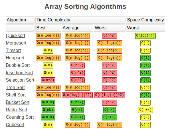
Preview of the Next Lesson

We saw that Quick Sort's performance hinges on choosing a good pivot. In our next lesson, we will dive deeper into this topic: Analyze pivot selection strategies in quick sort and its impact on average vs. worst-case performance. We'll explore strategies like picking a random element or the "median-of-three" to mitigate the risk of the dreaded $O(n^2)$ performance.