Two-Stage Recommender System Architecture

1. The Two-Stage Paradigm: Why Not Just Rank Everything? (Easy)

• Technical Explanation:
  Imagine a platform like YouTube, with billions of videos. For every user visiting the homepage, it's computationally impossible to evaluate every single video with a complex model to find the perfect recommendations. The latency would be minutes, not milliseconds.

  To solve this, modern recommendation systems use a two-stage "funnel" architecture:

  1. Candidate Generation (or Retrieval): This first stage acts as a coarse filter. Its job is to rapidly sift through the entire corpus of billions of items and select a few hundred plausible candidates (e.g., 500 videos) that are broadly relevant to the user. This stage prioritizes high recall (don't miss any potentially good items) and low latency.
  2. Ranking: This second stage takes the small set of candidates and uses a powerful, feature-rich, and computationally expensive model to score and rank them precisely. This stage prioritizes high precision (the top items on the list should be extremely relevant).

  This division of labor allows the system to deliver highly personalized recommendations from a massive catalog within strict latency budgets.

*This diagram from the original YouTube recommendation paper illustrates the funnel. Millions of items from the corpus are filtered by the Candidate Generation stage into hundreds, which are then meticulously scored and sorted by the Ranking stage to produce the final list of dozens shown to the user.*

• Metaphor for a 5-Year-Old:
  You're looking for a new toy in the world's biggest toy store.

  • Ranking Everything (The Slow Way): You could look at every single toy in the entire store, one by one, to decide which one you want most. You'd be there all day!
  • Two-Stage System (The Fast Way):
    1. Candidate Generation: You first run to the "Lego" section. You've instantly ignored all the dolls and board games, narrowing millions of toys down to just a few hundred Lego sets.
    2. Ranking: Now, you carefully look at the box art, piece count, and theme of each of the Lego sets in that aisle to pick the absolute best one.

• Anchor Resource:
  The original Google paper on YouTube's recommendation system is a foundational text. It clearly outlines the motivation for their two-stage design.

2. Candidate Generation: Finding Potential Needles in a Haystack (Medium)

• Technical Explanation:
  The goal of this stage is to learn low-dimensional vector representations (embeddings) for both users and items. The core idea is that if we map users and items to a shared embedding space, we can find relevant items for a user by finding item embeddings that are "close" to that user's embedding. The dominant architecture for this today is the Two-Tower Model.

  A two-tower model consists of:

  • Query Tower: A neural network that takes user features (e.g., watch history IDs, search query tokens, demographics) and outputs a single user embedding vector, $u\in {\mathbb{R}}^d$.
  • Item Tower: A separate neural network that takes item features (e.g., video ID, category) and outputs an item embedding vector, $v\in {\mathbb{R}}^d$.

  The model is trained on historical user-item interactions (e.g., user U watched video V). For a positive pair (U, V), the training objective is to maximize the similarity between their embeddings, typically measured by the dot product: $\text{similarity}(u,v)=u\cdot v$. For negative pairs (items the user did not interact with), the objective is to minimize this similarity.

• Metaphor for a 5-Year-Old:
  Imagine you have a magic map. The Item Tower is a machine that takes every food in the world and puts a magic sticker on the map for it (e.g., apples are here, pizza is there). The Query Tower is another machine that talks to you about what you like to eat and then puts a "You Are Here" sticker on the map for you. To find food you'll like, you just look for all the food stickers that are right next to your "You Are Here" sticker.

• Python Snippet (Simplified Two-Tower Model in PyTorch):
  This code shows the architectural skeleton. In a real system, the inputs would be more complex (e.g., bags of embeddings for watch history).

  import torch
  import torch.nn as nn
  
  class TwoTowerModel(nn.Module):
      def __init__(self, user_feature_dim, item_feature_dim, embedding_dim):
          super().__init__()
          
          # Query/User Tower
          self.user_tower = nn.Sequential(
              nn.Linear(user_feature_dim, 128),
              nn.ReLU(),
              nn.Linear(128, embedding_dim)
          )
          
          # Item Tower
          self.item_tower = nn.Sequential(
              nn.Linear(item_feature_dim, 128),
              nn.ReLU(),
              nn.Linear(128, embedding_dim)
          )
  
      def forward(self, user_features, item_features):
          # Generate embeddings
          user_embedding = self.user_tower(user_features)
          item_embedding = self.item_tower(item_features)
          
          # Normalize embeddings (good practice for cosine similarity)
          user_embedding = nn.functional.normalize(user_embedding, p=2, dim=1)
          item_embedding = nn.functional.normalize(item_embedding, p=2, dim=1)
          
          # Calculate dot product similarity for a batch
          # In a real training loop, you'd compare this to labels using a loss
          # like contrastive loss or binary cross-entropy on the logits.
          scores = torch.sum(user_embedding * item_embedding, dim=1)
          
          return scores
  
  # --- Example Usage ---
  EMBEDDING_DIM = 64
  model = TwoTowerModel(user_feature_dim=32, item_feature_dim=32, embedding_dim=EMBEDDING_DIM)
  
  # Fake batch of data: 4 users and 4 corresponding items they interacted with
  users = torch.randn(4, 32)
  items = torch.randn(4, 32)
  
  similarity_scores = model(users, items)
  print("Similarity scores for positive user-item pairs:")
  print(similarity_scores)
  

• Anchor Resource:
  To see this explained in the context of an interview, watch this mock interview segment where a candidate details the two-tower architecture.

3. The Ranking Stage: Finding the Sharpest Needle (Medium)

• Technical Explanation:
  Once candidate generation provides a list of ~500 items, the ranker's job is to score them with high precision. The key advantage here is that we can now afford to use a much richer feature set. The ranking model is typically a large, multi-layer feed-forward neural network (a.k.a. a Deep Neural Network or DNN).

  Crucial Distinctions of the Ranking Stage:

  • Rich Features: Unlike the candidate generator which might only use user/item IDs, the ranker uses hundreds of features:
    • Query Features: Time of day, device, user language.
    • Item Features: Content features (text, image embeddings), freshness ("Example Age" in the YouTube paper), popularity statistics.
    • User-Item Interaction Features: How many times has this user watched videos from this channel? When was the last time? These are extremely powerful signals.
  • Complex Objective Function: Simply predicting click-through rate (CTR) is naive. It promotes "clickbait." A better objective is to predict expected engagement. For YouTube, this is often expected watch time. This is cleverly implemented using a weighted logistic regression, where positive examples (clicks) are weighted by the actual watch time. The model's output $e^{Wx+b}$ then approximates expected watch time.
  • Model Architecture: The input layer takes all these diverse features. Categorical features are embedded, continuous features are normalized (and often powered, e.g., $x,x^2,\sqrt{x}$) to give the network more expressive power. These are then fed through several hidden layers (e.g., 1024 -> 512 -> 256 ReLU units).

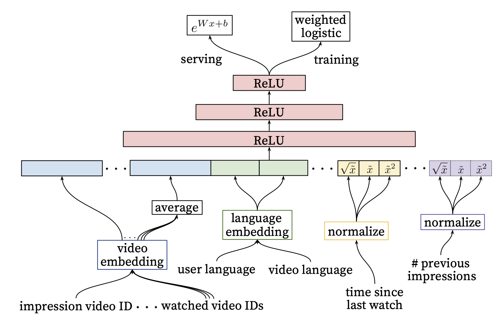
*This diagram shows a typical ranking model architecture. Note the variety of input features (embeddings for categorical, normalized values for continuous) being fed into a series of ReLU layers. This complex model is feasible because it only scores a few hundred items per request.*

• Metaphor for a 5-Year-Old:
  You have 10 final contestants for a talent show (the candidates). Now, a panel of three expert judges (the ranking model) comes out. They don't just ask "Can you sing?" (a single feature). They score each contestant on vocal quality, stage presence, costume, song choice, and audience reaction (many features). They combine all these scores to decide who is the absolute best performer (the top-ranked item).

• Anchor Resource:
  The YouTube paper provides an excellent, in-depth look at their ranking model.

4. Serving at Scale: The Online/Offline Dance (Hard)

• Technical Explanation:
  How do these two stages come together in a live production environment? It's a combination of offline batch processing and online real-time inference.

  • Offline System (Batch Jobs):

    1. The two-tower model and the ranking DNN are trained on massive datasets of user logs.
    2. The trained item tower is used to pre-compute embeddings for every single item in the corpus (millions/billions).
    3. These item embeddings are loaded into a specialized, high-performance index for fast lookups. This is not a standard database; it's an Approximate Nearest Neighbor (ANN) index (e.g., using libraries like ScaNN or FAISS). ANN allows you to find the "closest" vectors to a query vector in sub-linear time, making it possible to search millions of items in milliseconds.

  • Online System (Per User Request):

    1. A user request hits the server.
    2. The system fetches the user's features (e.g., recent watches, profile info) from a feature store.
    3. These features are fed into the query tower in real-time to generate a fresh user embedding.
    4. This user embedding is used as a query to the ANN index. The index returns the IDs of the top ~500 items whose embeddings are closest to the user's embedding. This completes the Candidate Generation stage.
    5. For these 500 candidate IDs, the system performs a batch lookup to fetch their full feature sets from a feature store.
    6. The ranking model scores all 500 candidates using their rich features.
    7. The final list is sorted by score. A post-processing step might apply business logic (e.g., filter watched items, ensure diversity).
    8. The final, ranked list is returned to the user.

• Metaphor for a 5-Year-Old:
  You're a librarian.

  • Offline: Overnight, you read every book in the library and create a master "topic" catalog (the ANN index) that lists which books are about space, which are about dinosaurs, etc.
  • Online: A child comes to you and says, "I love dinosaurs!" (the user query). You generate an idea of what they want ("dinosaurs", the user embedding). You instantly flip to the "dinosaurs" section in your master catalog (querying the ANN index) and pull out all 20 dinosaur books (candidates). Then, you quickly read the back covers of those 20 books (ranking) to recommend the one with the coolest pictures for that specific child.

• Anchor Resource:
  This article provides a fantastic overview of the end-to-end process, including the ANN search step.

5. Advanced Topics: Cold Starts, Bias, and Multi-Objective Ranking (Harder)

• Technical Explanation:
  A basic two-stage system is great, but elite systems must handle several complex challenges:

  1. The Cold Start Problem: How do you recommend to a new user (no interaction history) or recommend a brand-new item (no one has interacted with it yet)?
     • New User: Fall back on demographic features, geographic location, or simply show a globally popular set of items to gather initial signals.
     • New Item: Use its content features (text, images) to create an initial embedding. The item tower can be trained to handle this.
  2. Position Bias: Users naturally click on items at the top of a list more often, simply because they see them first. This pollutes your training data, making the model think top-ranked items are more relevant than they are.
     • Mitigation: A common technique is to include the item's position on the page as a feature during training. The model learns to associate a high position with a higher click probability. Then, during inference, this feature is removed or set to a default (e.g., position 1 for all candidates), forcing the model to rely only on the true relevance features.
  3. Multi-Objective Optimization: A business rarely has a single goal. You might want to optimize for watch time, and likes, and shares.
     • Solution: The ranking model can be designed with multiple "heads," where each head predicts a different objective. The final score is then a weighted combination of these predictions: Final Score = w1 * P(like) + w2 * P(share) + w3 * E(watch_time). The weights (w1, w2, w3) are tuned based on business priorities.

• Anchor Resource:
  This video on YouTube's more advanced ranking system directly addresses position bias and multi-objective ranking.

Conclusion

You now have a robust blueprint for designing a modern, large-scale recommendation system. This two-stage architecture is a powerful and proven pattern for tackling the immense scale of today's platforms.

Key Takeaways:

• Recommendation at scale is a two-stage problem: fast, high-recall candidate generation followed by a precise, feature-rich ranking stage.
• Two-Tower models are the industry standard for learning user and item embeddings for candidate generation.
• Ranking models are powerful DNNs that leverage hundreds of features and optimize for complex business objectives like expected watch time, not just clicks.
• The entire system is orchestrated through an online/offline design, where item embeddings are pre-computed and stored in an ANN index for low-latency retrieval during a user request.
• Elite systems must also thoughtfully address challenges like cold start, biases in the data, and balancing multiple objectives.

Next Lesson Preview

In this lesson, we discussed that candidate retrieval is powered by an Approximate Nearest Neighbor (ANN) index that can search millions of embeddings in milliseconds. But how do these indexes work? What are their internal data structures and trade-offs? In our final content lesson for this module, we will dive deep into this critical piece of infrastructure and learn how to design the architecture of a scalable vector database using Approximate Nearest Neighbor (ANN) indexing.