Model Optimization for Efficient Deployment

1. The Efficiency Imperative: Why Bigger Isn't Always Better (Easy)

• Technical Explanation:
  In a production environment, a model's "goodness" is not solely defined by its accuracy. Three other critical metrics dictate its viability:

  • Inference Latency: The time taken to produce a single prediction. For real-time applications like ad ranking or type-ahead search, this must be in the order of milliseconds.
  • Throughput: The number of predictions the system can serve per second. Higher throughput means you can serve more users with the same hardware.
  • Memory Footprint & Cost: The amount of RAM/VRAM a model occupies. Large models require more expensive hardware (e.g., GPUs with more VRAM) and more servers, directly increasing operational costs.

  Often, a marginal gain in accuracy from a larger model is not worth the significant increase in cost and latency. The goal of model optimization is to find the "sweet spot" on the accuracy-efficiency curve that meets both business objectives and performance budgets.

• Metaphor for a 5-Year-Old:
  You have two cars for delivering pizza. One is a giant, super-fast Formula 1 race car (Large Model). It's the fastest car in the world (high accuracy), but it uses special, expensive fuel (high cost), needs a huge garage (high memory), and is tricky to start (high latency). The other car is a nimble scooter (Optimized Model). It's not the absolute fastest, but it's cheap to run, easy to park anywhere, and can zip through traffic to deliver pizzas quickly and reliably for most customers. For a pizza delivery business, the scooter is often the better choice.

• Anchor Resource & Real-World Example:
  The challenge of balancing accuracy and efficiency is not new. The famous Netflix Prize competition provides a classic cautionary tale.

2. Knowledge Distillation: Learning from a "Teacher" Model (Medium)

• Technical Explanation:
  Knowledge Distillation is a technique where we use a large, complex, and highly accurate model (the "teacher") to train a smaller, more efficient model (the "student"). The key insight, pioneered by Geoffrey Hinton, is that the teacher model's full output probability distribution (the "soft labels" or logits) contains more information than the simple ground-truth "hard label".

  For example, when classifying an image of a cat, the teacher might output: {Cat: 90%, Dog: 8%, Car: 2%}. This tells the student that a cat looks a bit like a dog, but not at all like a car. The student is trained to mimic this nuanced output. The training loss for the student is a weighted average of two components:

  1. Distillation Loss: Measures how well the student's soft labels match the teacher's soft labels (often using Kullback-Leibler Divergence).
  2. Student Loss: The standard loss function comparing the student's predictions to the hard ground-truth labels (e.g., Cross-Entropy).

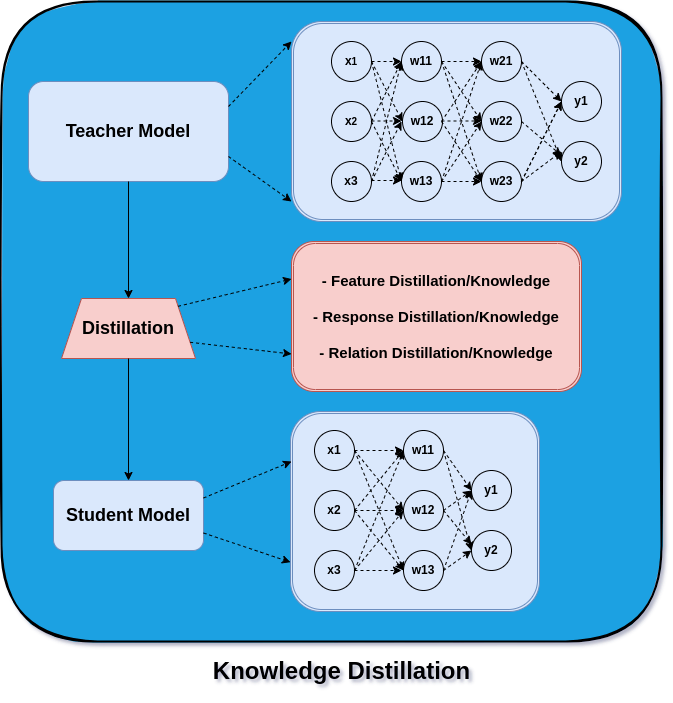
*This diagram illustrates the Knowledge Distillation framework. A larger Teacher Model transfers its learned 'knowledge' (in the form of response, feature, or relation distributions) to a smaller, more efficient Student Model.*

• Metaphor for a 5-Year-Old:
  A master chef (teacher) is teaching a junior cook (student) how to bake a cake.

  • Hard Labels: The chef could just give the student a recipe that says "bake for 30 minutes".
  • Soft Labels: Instead, the chef says, "Bake it until it's golden brown, smells nutty, and a toothpick comes out clean. It usually takes about 30 minutes, but it might be 28 if the oven is hot or 32 if the eggs were cold." The student learns the reasoning behind the decision, not just the final answer, and becomes a better cook.

• Industry Example: Meta's Ad Models
  Meta uses this exact technique at a massive scale. Their giant "Generalized Ad Model" (GEM) acts as a teacher for hundreds of smaller, specialized "Vertical Models" (VMs) that are fast enough to serve ads in real-time on products like Instagram Stories.

3. Quantization: Speaking the Language of Hardware (Medium)

• Technical Explanation:
  Quantization is the process of reducing the numerical precision of a model's weights and/or activations. Most models are trained using 32-bit floating-point numbers (FP32). Quantization converts these numbers to a lower-precision format, most commonly 8-bit integers (INT8).

  This has two major benefits that go right to the hardware level:

  1. Reduced Memory: An INT8 value uses 4x less memory than an FP32 value. This means your model's size is reduced by roughly 75%, and you use less memory bandwidth to load the weights.
  2. Faster Computation: CPUs and GPUs can perform integer arithmetic much faster than floating-point arithmetic. Modern AI accelerators (like NVIDIA's Tensor Cores) have specialized INT8 hardware that dramatically boosts throughput.

  To convert from FP32 to INT8, we need a mapping function. For each layer or tensor, we find the minimum and maximum FP32 values and map this range to the INT8 range (e.g., -127 to 127). This mapping is defined by two parameters:

  • Scale (s): A float that determines the step size of the mapping.
  • Zero-point (z): An integer that ensures the real value zero maps correctly to a quantized value.

  The formula is: $real\_value=scale\times (quantized\_value-zero\_point)$

• Metaphor for a 5-Year-Old:
  You're drawing a picture with a giant box of 16 million crayons (FP32), where you have every possible shade of every color. It's very precise, but carrying the box is slow. Quantization is like choosing a smaller box of just 256 essential crayons (INT8). You can draw the same picture much faster, and for most people, it will look just as good. The scale and zero-point are your guide for picking the closest crayon from the small box to match a color from the big box.

• Anchor Resource:
  To truly understand quantization, it's helpful to see the mechanics. This video provides an excellent, detailed explanation with PyTorch examples.

4. Implementing Quantization: Post-Training vs. Aware Training (Hard)

• Technical Explanation:
  There are two main strategies for applying quantization:

  1. Post-Training Quantization (PTQ): This is the simplest method. You take a fully-trained FP32 model and convert its weights to INT8 after training. To determine the scale and zero-point for activations (which change with every input), you need to run a small, representative "calibration" dataset through the model to observe their range.

     • Pros: Fast, easy, no retraining required.
     • Cons: Can lead to a noticeable drop in accuracy, as the model was never trained to handle precision loss.

  2. Quantization-Aware Training (QAT): This method simulates the effects of quantization during the training process. "Fake quantize" nodes are inserted into the model graph. During the forward pass, they quantize and then de-quantize the weights and activations, forcing the model to learn to be robust to the rounding errors. The backpropagation still happens in FP32.

     • Pros: Almost always results in higher accuracy than PTQ, sometimes with no loss at all.
     • Cons: Requires retraining or fine-tuning, which is more complex and time-consuming.

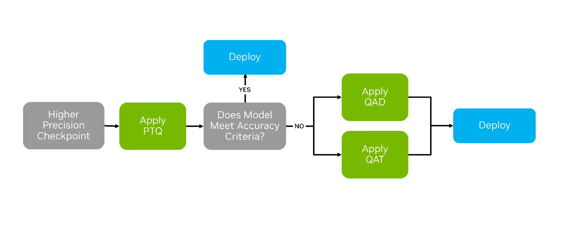
*This flowchart illustrates a common decision process. Start with PTQ. If accuracy criteria are not met, proceed to more complex methods like QAT or Quantization-Aware Distillation (QAD).*

• Python Snippet (Dynamic PTQ in PyTorch):
  PyTorch provides excellent tools for quantization. Here’s how you would apply dynamic PTQ—the simplest form where weights are quantized offline and activations are quantized on-the-fly.

  import torch
  import torch.nn as nn
  import os
  
  # 1. Define a simple FP32 model (assume it's already trained)
  class SimpleModel(nn.Module):
      def __init__(self):
          super(SimpleModel, self).__init__()
          self.fc1 = nn.Linear(10, 20)
          self.relu = nn.ReLU()
          self.fc2 = nn.Linear(20, 5)
      
      def forward(self, x):
          x = self.fc1(x)
          x = self.relu(x)
          x = self.fc2(x)
          return x
  
  # Create an instance of the trained model
  trained_fp32_model = SimpleModel()
  # In a real scenario, you would load your trained weights here
  # trained_fp32_model.load_state_dict(torch.load('trained_model.pth'))
  trained_fp32_model.eval()
  
  # 2. Apply Post-Training Dynamic Quantization
  # This command automatically converts the specified linear layers to use INT8 weights
  # and calculates activations dynamically.
  quantized_model = torch.quantization.quantize_dynamic(
      model=trained_fp32_model,
      qconfig_spec={nn.Linear},  # Specify which layers to quantize
      dtype=torch.qint8          # Target data type
  )
  
  # 3. Compare model sizes
  def print_model_size(model, label):
      torch.save(model.state_dict(), "temp.p")
      size_mb = os.path.getsize("temp.p")/1e6
      print(f"Size of {label}: {size_mb:.2f} MB")
      os.remove("temp.p")
  
  print_model_size(trained_fp32_model, "FP32 Model")
  print_model_size(quantized_model, "Quantized INT8 Model")
  
  # Example usage: The quantized model works just like the original
  input_fp32 = torch.randn(1, 10)
  output = quantized_model(input_fp32)
  print("\nQuantized model output:", output)
  

5. Designing a Production Optimization Strategy (Harder)

• Technical Explanation:
  Given these techniques, how do you decide which one to use? A pragmatic, iterative approach is best, balancing engineering effort with performance gains.

  1. Establish a Baseline: First, benchmark your FP32 model's accuracy and performance (latency, throughput). Define your targets (e.g., "p99 latency < 50ms" and "accuracy drop < 1%").
  2. Attempt PTQ: Always start with Post-Training Quantization. It's the "low-hanging fruit". Calibrate your model and measure its accuracy and performance. If it meets your targets, you're done! Deploy it.
  3. Move to QAT: If the accuracy drop from PTQ is too severe, your next step is Quantization-Aware Training. Fine-tune your model for a few epochs with QAT enabled. This requires more effort but usually recovers the lost accuracy.
  4. Consider Knowledge Distillation: If your model is architecturally too complex (e.g., has too many layers or parameters) and even a quantized version is too slow or large, use Knowledge Distillation. Train a completely new, smaller student model from scratch, using your original model as the teacher.
  5. Combine Techniques: These methods are not mutually exclusive. A powerful strategy is to first use distillation to get from a massive teacher to a manageable student, and then use QAT to quantize that student model for maximum efficiency.

  Other techniques like Pruning (removing redundant weights) and Low-Rank Factorization (decomposing weight matrices) also exist and can be integrated into this flow, but distillation and quantization are often the most impactful starting points.

• Metaphor for a 5-Year-Old:
  You need to fit your toys into a small backpack for a trip.

  1. Baseline: You see how many toys you have and which ones are your favorites.
  2. PTQ: You try to squish your stuffed animals into the bag. It's fast, but some might get misshapen.
  3. QAT: You go back and get special "travel" stuffed animals that are designed to be squished and pop back into shape perfectly.
  4. Distillation: You look at your giant toy castle and realize it will never fit. Instead, you take a few of your favorite knight and dragon figures that let you play the same games, but take up way less space.
  5. Combine: You take just the knight and dragon figures (Distillation) and you make sure they are the squishable travel kind (Quantization).

Conclusion

You have now learned the critical techniques for bridging the gap between a high-accuracy prototype and a high-performance production model. Efficiency is not an afterthought; it is a core requirement for building scalable and cost-effective AI systems.

Key Takeaways:

• Model optimization is a crucial step to balance accuracy with production constraints like latency, throughput, and cost.
• Knowledge Distillation allows a small "student" model to learn the rich, nuanced patterns from a large "teacher" model, enabling significant architectural simplification.
• Quantization drastically reduces model size and speeds up computation by converting weights from FP32 to lower-precision formats like INT8, leveraging hardware-level optimizations.
• There's a clear workflow for optimization: start with the simplest method (PTQ), and if accuracy suffers, move to more robust but complex methods like QAT or Distillation.

Next Lesson Preview

With this module on MLOps complete, we will now shift focus to a different but equally important aspect of becoming an elite engineer: communication and professional conduct. In the next lesson, we will begin the "Interview Readiness" module and learn how to apply the STAR method to structure responses for behavioral questions about leadership, conflict, and failure.