Scalable Vector Database Architecture with ANN Indexing

1. Why a Specialized Vector Database? (Easy)

• Technical Explanation:
  As we saw in the last lesson, embedding models (like the two towers) convert complex data like text, images, or user behavior into high-dimensional numerical vectors. The key property of these embeddings is that semantic similarity corresponds to spatial proximity. In other words, vectors for similar concepts are close to each other in the vector space.

  A vector database is a database system specifically designed to store, manage, and query these high-dimensional vector embeddings efficiently.

  Why can't we just use a traditional SQL or NoSQL database?

  • Lack of Dimensionality Understanding: Traditional databases are optimized for filtering on exact values (e.g., WHERE country = 'USA') or ranges on low-dimensional data (e.g., WHERE price > 100). They have no built-in concept of "find me the closest vectors to this query vector" in a 128- or 768-dimensional space.
  • Inefficient Search: A traditional database would have to perform a "full table scan," calculating the distance between the query vector and every single vector in the database. This brute-force approach is computationally infeasible for millions or billions of items.

  Vector databases solve this by integrating specialized indexing structures—known as ANN indexes—directly into the query engine.

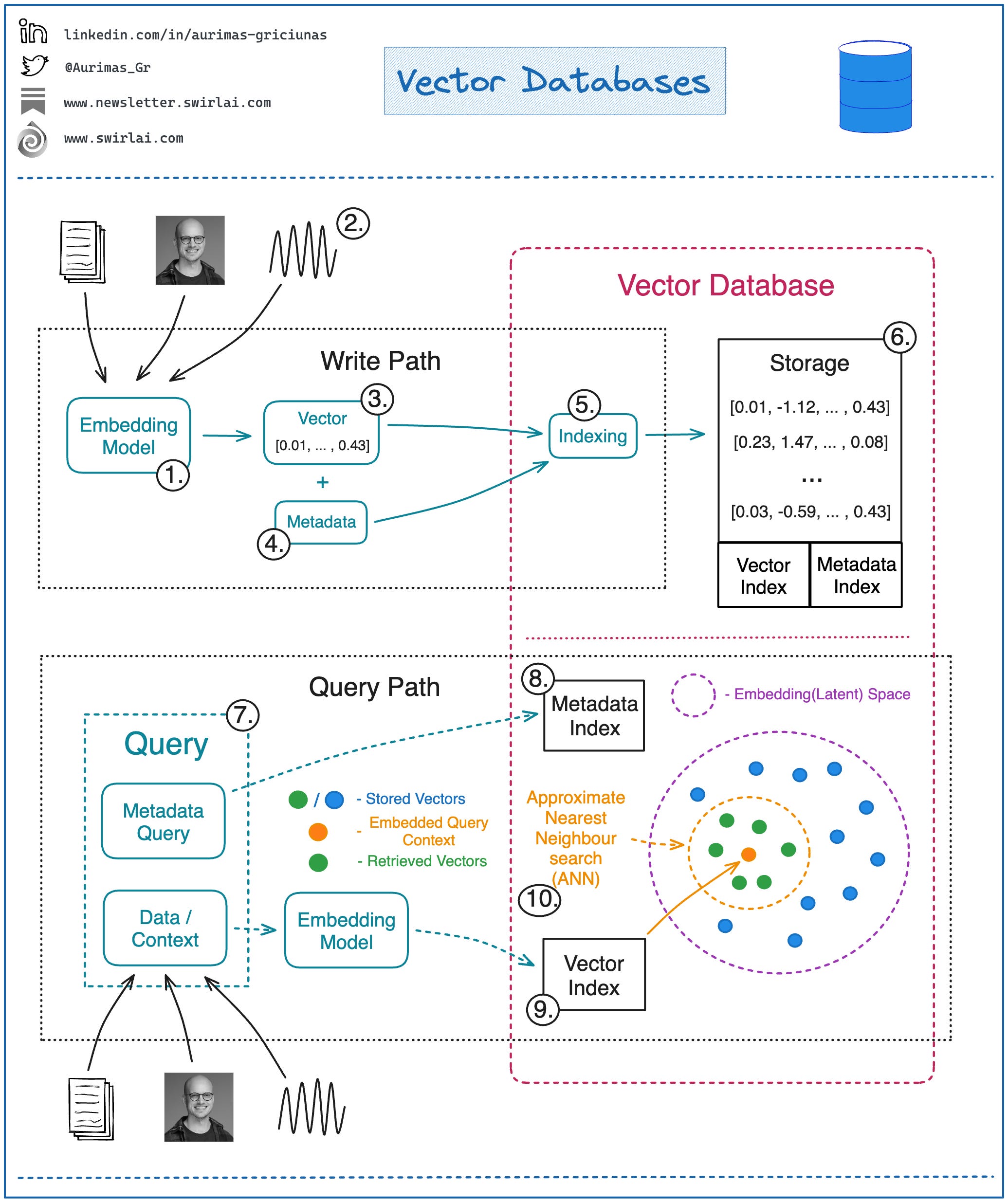
*This diagram shows the two main workflows in a vector database. The **Write Path** (top) takes raw data, embeds it, and places it in an index. The **Query Path** (bottom) embeds a query, then uses an ANN search algorithm to find the most similar vectors from the index.*

• Metaphor for a 5-Year-Old:
  Imagine you have a giant box of Lego bricks of all different colors.

  • Traditional Database: This is like organizing the bricks into small, labeled drawers: "Red 2x4s," "Blue 1x1s," etc. It's great if you need exactly a "Red 2x4." But if you need a brick that is "sort of reddish-orange," you'd have to open every single drawer to find the best match.
  • Vector Database: This is like dumping all the bricks onto a giant mat where you've magically arranged them so that all the red bricks are in one corner, all the blues in another, and the oranges and yellows are in between the reds and yellows. If you want a "reddish-orange" brick, you just go to the area on the mat between the red and yellow corners to instantly find all the best candidates.

• Anchor Resource:
  Let's start with a clear, high-level overview of what vector databases are and why they are essential for modern machine learning applications, especially Large Language Models (LLMs).

2. The Core Trade-off: Exact vs. Approximate Search (Medium)

• Technical Explanation:
  The fundamental task in a vector database is k-Nearest Neighbor (k-NN) search: given a query vector $q$, find the $k$ vectors in the database that are "closest" to it.

  Similarity Metrics: "Closeness" is measured using a distance function. The most common are:

  • Euclidean Distance (L2): The straight-line distance between two points. $d(a,b)=\sqrt{{\sum }_{i=1}^D(a_i-b_i{)}^2}$. Best for when magnitude matters.
  • Cosine Similarity: The cosine of the angle between two vectors. It measures orientation, not magnitude. It's often calculated from dot product on normalized vectors. $\text{similarity}(a,b)=\frac{a\cdot b}{\Vert a\Vert \Vert b\Vert }$. Best for text embeddings where direction captures meaning.
  • Dot Product: Can be used for similarity if vectors are normalized. If not, it's influenced by both magnitude and angle.

  Exact k-NN (Brute Force): The only way to guarantee you find the exact nearest neighbors is to compute the distance from the query vector $q$ to every other vector in the database. With $N$ vectors of dimension $D$, the time complexity is $O(N\cdot D)$. For a billion vectors ($N=10^9$), this is prohibitively slow for real-time applications.

  Approximate k-NN (ANN): This is the key idea behind vector databases. Instead of guaranteeing the perfect answer, we build a clever index that allows us to find very close neighbors extremely quickly. We trade a small amount of accuracy for a massive gain in speed.

  • Recall: The primary metric for an ANN index is recall@k. It measures what fraction of the true top-k neighbors were found by the approximate search. A recall of 95% means the ANN search returned 95% of the actual top-k items.
  • The Trade-off: The core challenge in designing and tuning a vector database is balancing the "iron triangle" of Recall, Query Speed (QPS), and Memory Usage.

• Metaphor for a 5-Year-Old:
  You lost your favorite red marble in a giant sandbox with a million other marbles.

  • Exact Search: You sift through the entire sandbox, one handful at a time, comparing every single marble to the picture of your lost one. You'll find it, but it will take all day.
  • Approximate Search: You know your marble is red. So you only search in the parts of the sandbox where you see other red marbles. You might accidentally miss your marble if it rolled into the blue marble area, but you'll finish searching in 5 minutes and will most likely find one that looks almost identical.

• Anchor Resource:
  This video explains the need for indexing and introduces different similarity metrics.

3. A Survey of ANN Indexing Algorithms (Medium)

• Technical Explanation:
  ANN algorithms build a data structure (the index) that can be searched much faster than a linear scan. There are several families of algorithms, each with different trade-offs.

  1. Hashing-Based (e.g., Locality-Sensitive Hashing - LSH): The core idea is to devise hash functions such that similar vectors have a high probability of colliding into the same hash bucket. To find neighbors for a query vector, you hash it and then only compare distances with the vectors in the same bucket. It's one of the earliest methods but is often outperformed in practice by modern graph or tree-based indexes.

  2. Tree-Based (e.g., Annoy from Spotify): These methods recursively partition the vector space using hyperplanes. The data is partitioned into a set of trees. A search involves traversing the trees to find the leaf nodes that are closest to the query vector. It's simple and memory-efficient but can struggle with very high-dimensional data.

  3. Quantization-Based (e.g., Product Quantization - PQ): These methods focus on compressing the vectors to reduce their memory footprint and speed up distance calculations. Product Quantization, for instance, breaks a large vector into smaller chunks, runs a clustering algorithm (like k-means) on each set of chunks to create "codebooks," and then represents each vector as a short code of cluster IDs. Search can then be done on these compressed codes. PQ is often used in combination with other index types.

  4. Graph-Based (e.g., HNSW, NSG, DiskANN): These are currently the state-of-the-art for many high-performance use cases. The idea is to build a graph where each node is a vector, and edges connect nodes to their nearest neighbors. A search is performed by "navigating" the graph, starting from a random or fixed entry point and greedily moving towards the query vector. Hierarchical Navigable Small World (HNSW) is one of the most popular and powerful graph-based algorithms.

• Metaphor for a 5-Year-Old:
  How do you find a friend's house in a big city?

  • Hashing: All friends living on "Main Street" have to go to the same playground. You go to the "Main Street" playground to find your friend.
  • Tree: You ask a series of questions: "Does my friend live north or south of the river?" (South). "East or west of the park?" (East). You keep narrowing down the area.
  • Graph: Everyone knows their immediate neighbors. You start at your house, ask your neighbor "Which way to John's house?". They point you to the next neighbor in the right direction, and you keep asking until you arrive.

• Anchor Resource:
  The video from The ML Tech Lead! gives a good high-level intuition for several of these methods.

4. Deep Dive: Hierarchical Navigable Small World (HNSW) (Hard)

• Technical Explanation:
  HNSW is the dominant algorithm for in-memory ANN search due to its excellent performance. It combines two key ideas: the Navigable Small World graph and the multi-layer hierarchy of a skip list.

  1. Navigable Small World (NSW): An NSW graph connects each vector (node) to its nearest neighbors. Some of these are short-range links (connecting very close points) and some are long-range links (connecting distant points). This structure allows for fast traversal across the graph. The problem is that greedy search can get stuck in a "local minimum" and miss the true nearest neighbor.

  2. The Hierarchy: HNSW improves on NSW by building multiple layers of graphs.

     • The bottom layer (Layer 0) contains all the vectors, with dense, short-range connections.
     • Each subsequent layer above it is a sparse sub-graph of the layer below. A vector is added to a higher layer with a declining probability.
     • The top layer is very sparse, containing only a few nodes with long-range connections that act as fast "highways" across the vector space.

*This illustrates the HNSW search process. The search starts at an entry point in the sparsest top layer (Layer 2). It greedily navigates to the closest point to the query in that layer. It then drops down to the next layer (Layer 1), using the best point from above as the new starting point. This process repeats until it finds the local minimum in the densest bottom layer (Layer 0), which is the final result.*

**Key Hyperparameters & Trade-offs:**
*   `m`: The number of neighbors each node will be connected to. Higher `m` increases index size and build time but improves recall.
*   `efConstruction`: The size of the dynamic candidate list during index construction. A larger value creates a higher quality graph (better recall) but makes indexing much slower.
*   `efSearch`: The size of the candidate list during a search. This is the most important query-time parameter. Higher `efSearch` increases accuracy/recall at the cost of lower QPS (slower queries).

• Python Snippet (Using Faiss for HNSW):
  Faiss (Facebook AI Similarity Search) is a standard library for vector search. This snippet shows how to build a basic HNSW index.

  import numpy as np
  import faiss
  
  # 1. Setup
  d = 128      # Vector dimension
  N = 100000   # Number of vectors in the database
  k = 5        # Number of nearest neighbors to find
  
  # Generate some random data
  np.random.seed(42)
  db_vectors = np.float32(np.random.random((N, d)))
  query_vectors = np.float32(np.random.random((10, d)))
  
  # 2. Build the HNSW index
  # The 'm' parameter is the number of connections per node
  m = 32  
  index = faiss.IndexHNSWFlat(d, m)
  
  # Set the efConstruction parameter (higher is slower but more accurate index)
  index.hnsw.efConstruction = 40
  print("Building HNSW index...")
  index.add(db_vectors)
  print(f"Index is trained: {index.is_trained}")
  print(f"Total vectors in index: {index.ntotal}")
  
  # 3. Search the index
  # Set the efSearch parameter (higher is more accurate but slower search)
  index.hnsw.efSearch = 16
  print("\nSearching for k-nearest neighbors...")
  distances, indices = index.search(query_vectors, k)
  
  # 4. Display results for the first query
  print(f"\nResults for the first query vector:")
  print(f"Nearest neighbor indices: {indices[0]}")
  print(f"Distances (L2): {distances[0]}")
  

• Anchor Resource:
  This video provides a phenomenal, in-depth explanation of HNSW, including its implementation in Faiss and the impact of its parameters.

5. Architecting a Scalable, Cloud-Native Vector Database (Harder)

• Technical Explanation:
  An ANN index like HNSW is the heart of a vector database, but a full-fledged, scalable system requires much more. Drawing from modern designs like Milvus (open-source) or Pinecone, a robust architecture separates concerns into a set of decoupled microservices.

  A cloud-native vector database architecture typically consists of four layers:

  1. Access Layer (Stateless Proxies): This is the user-facing entry point. Proxies receive API requests, perform basic validation, route requests to the appropriate internal services, and aggregate final results. Being stateless allows them to be scaled out easily.

  2. Coordinator Layer (The Brains): This layer consists of several coordinator services that manage the system's state and metadata.

     • Root Coordinator: Handles data definition (e.g., create/delete collections).
     • Query Coordinator: Manages the distribution of data segments across query nodes for load balancing.
     • Index Coordinator: Manages index-building tasks, dispatching them to index nodes.
     • Data Coordinator: Manages the flow of data from ingestion to persistent storage.

  3. Worker Layer (The Muscle): These are stateless compute nodes that perform the heavy lifting. They are decoupled and can be scaled independently.

     • Query Nodes: Load data segments and their indexes into memory to perform ANN searches.
     • Index Nodes: Receive tasks from the Index Coordinator to build indexes on new data segments.
     • Data Nodes: Ingest data, subscribe to a log stream, batch incoming writes, and persist data segments to object storage.

  4. Storage Layer (Persistence):

     • Object Storage (e.g., S3, MinIO): Used for storing bulk data like raw vectors, indexes, and logs due to its low cost and high durability.
     • Key-Value Store (e.g., etcd): Used to store system metadata, which needs high availability and strong consistency.

  The Log Backbone: A crucial design pattern is to use a distributed log (like Kafka or Pulsar) as the system's backbone. All data mutations (inserts, deletes) are first written to the log. Worker nodes then subscribe to this log to receive updates. This decouples the write path from the read path, enabling independent scaling and tunable consistency (users can query data that is still in the log before it's even indexed).

  Handling Updates and Large Datasets:

  • Segmenting: Instead of a single, massive, mutable index, data is broken into smaller, immutable segments. New data is written to a "growing" segment. Once it's full, it's "sealed," and an Index Node builds an index for it in the background. This avoids costly in-place updates to a giant index.
  • Quantization & Disk-Based Indexes: To handle billion-scale datasets that don't fit in RAM, systems use techniques like Product Quantization (PQ) to compress vectors. For even larger scale, indexes like DiskANN are designed to reside on SSDs, keeping only a small portion of the index or compressed codes in RAM.

• Anchor Resource:
  The paper on Manu (which became Milvus 2.0) is a masterclass in cloud-native database design and perfectly illustrates these architectural principles. The slides on advanced indexing cover strategies for handling large, dynamic datasets.

Conclusion

Congratulations, you've now gone from a user of ANN indexes in a recommendation system to an architect who understands how to build the entire vector database from first principles.

Key Takeaways:

• Vector databases exist to solve the unique problem of searching for semantic similarity in high-dimensional spaces, a task traditional databases are not built for.
• The core of a vector database is an ANN index, which makes a critical trade-off: sacrificing perfect accuracy for massive gains in query speed.
• HNSW is a state-of-the-art graph-based algorithm that provides excellent performance by building a multi-layered graph, enabling fast traversal from coarse to fine-grained results.
• A truly scalable vector database is a decoupled, cloud-native system with separate services for ingestion, indexing, querying, and coordination, often orchestrated via a log backbone.
• Handling billion-scale datasets requires advanced techniques like sharding, quantization, and disk-resident indexes, while handling real-time updates requires segmenting and liveness layers.

Next Lesson Preview

We have now completed the core modules on advanced algorithms and ML systems design. You've covered everything from fundamental data structures to the architecture of recommendation engines and vector databases. The final module of this course, "Interview Readiness and Practical Application," is about consolidating this knowledge and applying it under pressure.

In our next lesson, we will begin this final phase by learning how to apply the STAR method to structure responses for behavioral questions about leadership, conflict, and failure. While technical depth is crucial, your ability to communicate your experience and impact effectively is what separates a great engineer from an elite one.