Divide and Conquer: Mergesort & Quicksort

1. The Divide and Conquer Paradigm, Formalized

At its core, Divide and Conquer is a three-step process for solving problems.

To solidify this definition, let's turn to a more formal description.

As you can see, the strategy is:

1. Divide: Break the main problem into several smaller, independent subproblems.
2. Conquer: Solve the subproblems recursively. If a subproblem is small enough (the "base case"), solve it directly.
3. Combine: Merge the solutions of the subproblems to form the solution for the original problem.

In binary search, the "divide" was finding the midpoint, "conquer" was comparing the target to the midpoint's value, and "combine" was non-existent because we simply discarded the other half. For sorting, the "combine" step becomes much more interesting.

2. Mergesort: The Quintessential D&C Algorithm

Mergesort is a perfect illustration of the Divide and Conquer paradigm because its "Divide" and "Combine" steps are very distinct.

• Divide: The array is recursively split in half until we are left with subarrays of size 1. An array with one element is, by definition, already sorted. This is our base case.
• Conquer: This step is implicitly handled by the recursion reaching the base case.
• Combine: This is where the real work happens. We take two adjacent, sorted subarrays and merge them into a single, larger sorted subarray. This process is repeated up the recursion tree until the entire array is a single sorted unit.

The image below gives a fantastic visual of this entire process.

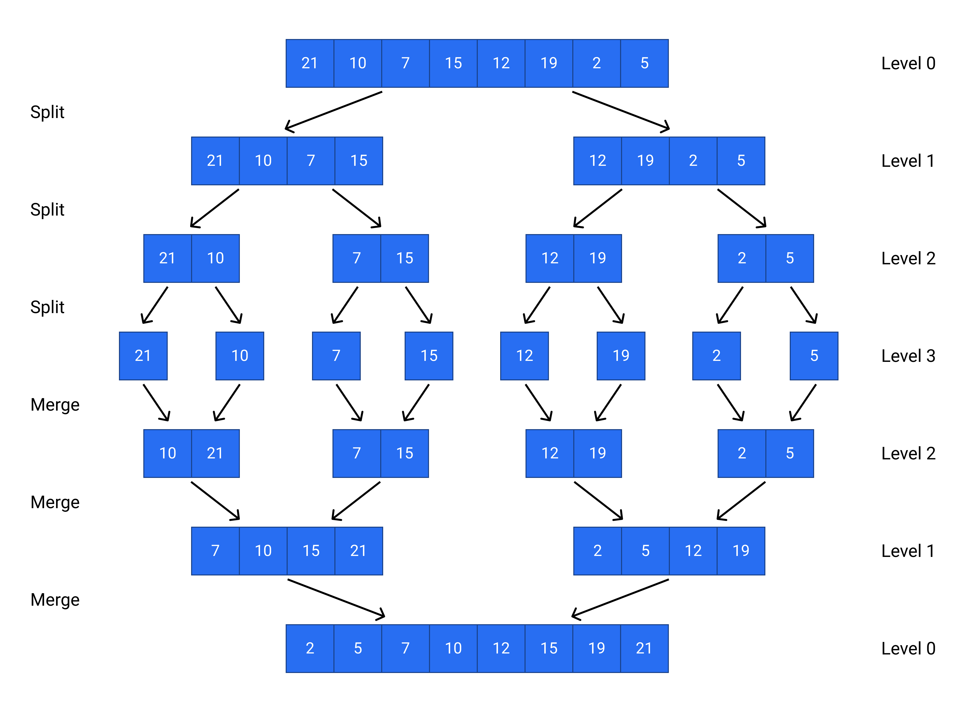
To truly understand the mechanics, especially the crucial merge step, let's watch a detailed explanation.

The Merge Subroutine

As the video demonstrated, the heart of Mergesort is the merge function. It takes two sorted subarrays and combines them. Here's the key logic:

1. Create a temporary array to hold the merged result. This means Mergesort is not an in-place algorithm and requires extra memory.
2. Use two pointers, one for each subarray, starting at the beginning of each.
3. Compare the elements at the two pointers. Copy the smaller element to the temporary array and advance its pointer.
4. Repeat until one subarray is exhausted.
5. Copy any remaining elements from the non-exhausted subarray into the temporary array.
6. Finally, copy the entire sorted temporary array back over the original segment.

Complexity Analysis of Mergesort

The analysis of Mergesort is a classic example of analyzing a recursive algorithm. The recurrence relation is:
$T(n)=2T(n/2)+O(n)$
This translates to: "The time to sort n elements, $T(n)$, is twice the time to sort n/2 elements (the two recursive calls), plus the linear time $O(n)$ required to merge those two halves."

As you may recall from our earlier lessons and the Master Theorem, this recurrence solves to $O(n\log n)$. The video you just watched provides a brief derivation of this.

The most important takeaways from an architectural standpoint are:

• Time Complexity: Mergesort's performance is a guaranteed $O(n\log n)$ in the best, average, and worst cases. This predictability is extremely valuable for systems where performance guarantees are critical.
• Space Complexity: It requires $O(n)$ auxiliary space for the temporary array used in merging. This can be a significant drawback for memory-constrained systems.

3. Quicksort: A Different D&C Philosophy

Quicksort is another famous sorting algorithm based on Divide and Conquer, but it flips the script on where the work is done.

• Mergesort: Trivial "Divide", complex "Combine".
• Quicksort: Complex "Divide", trivial "Combine".

Here's how Quicksort works:

1. Divide: This is the core step, called partitioning.
   • Choose an element from the array, called the pivot.
   • Reorder the array so that all elements with values less than the pivot come before it, while all elements with values greater than the pivot come after it. After this partitioning, the pivot is in its final sorted position.
2. Conquer: Recursively apply Quicksort to the sub-array of elements with smaller values and the sub-array of elements with larger values.
3. Combine: Do nothing! Because the pivot is already in its correct place and the subarrays are sorted independently, the entire array becomes sorted once the recursion finishes.

Let's get an intuition for this partitioning step.

Complexity Analysis of Quicksort: The Trade-off

This is where Quicksort differs most from Mergesort. Its performance depends heavily on the choice of the pivot.

• Best/Average Case: If the pivot consistently divides the array into roughly equal halves, the recurrence is $T(n)=2T(n/2)+O(n)$ (for partitioning), which again solves to $O(n\log n)$.
• Worst Case: What if we always pick the smallest or largest element as the pivot? This happens if you use a naive strategy (e.g., always pick the first element) and the array is already sorted. The partition will be extremely unbalanced: one sub-problem of size 0 and another of size $n-1$. This leads to the recurrence $T(n)=T(n-1)+O(n)$, which results in a dismal $O(n^2)$ time complexity.

This contrast between best and worst-case performance is a critical concept.

In practice, the worst-case is avoided by using a smarter pivot selection strategy, such as picking a random element. This makes the probability of hitting the worst-case scenario astronomically low, and gives Quicksort an expected time complexity of $O(n\log n)$. Most standard library implementations of sorting use a highly optimized version of Quicksort (often an introspective sort that switches to heapsort for pathological cases) because it is typically faster in practice and can be done in-place, using only $O(\log n)$ space for the recursion call stack.

Conclusion

In this lesson, we dissected the Divide and Conquer paradigm using two fundamental sorting algorithms. We've moved beyond just implementing algorithms to analyzing and comparing their architectural trade-offs—a key part of developing a senior engineering mindset.

Key Takeaways:

• Divide and Conquer is a powerful paradigm that involves breaking a problem into smaller subproblems, solving them recursively, and combining the results.
• Mergesort is a "pure" D&C algorithm with a trivial divide and a complex combine (merge). It offers guaranteed $O(n\log n)$ performance but requires $O(n)$ extra space.
• Quicksort has a complex divide (partition) and a trivial combine. It has an average-case $O(n\log n)$ performance but a worst-case of $O(n^2)$. It is typically implemented in-place, making it more space-efficient.
• The choice between them is a classic engineering trade-off: guaranteed performance vs. better average-case speed and lower memory usage.

Preview of the Next Lesson:

We have now seen how to solve problems by breaking them down and building them back up. In our next lesson, we will explore a completely different strategy: the Greedy paradigm. We'll learn how to solve optimization problems by making a sequence of locally optimal choices, and we'll analyze when this "short-sighted" approach can successfully lead to a globally optimal solution.