Hello! Welcome to our third lesson in the Algorithmic Design Paradigms module.
In our last session, we explored the Divide and Conquer paradigm through Mergesort and Quicksort. We saw how breaking a problem into independent subproblems and then combining their solutions is a powerful strategy. A key takeaway was analyzing the trade-offs, such as Mergesort's guaranteed performance versus Quicksort's superior space efficiency and average-case speed.
Today, we shift our focus to a completely different design philosophy: the Greedy paradigm. Instead of breaking down the problem first, this approach builds a solution step-by-step, making the most appealing choice at each moment. Your goal for this lesson is to explain the Greedy paradigm and the conditions for its applicability (greedy-choice property, optimal substructure). Understanding these conditions is crucial for an architect's mindset, as it's about knowing when and why a particular strategy is the right tool for the job.
1. What is a Greedy Algorithm?
A greedy algorithm constructs a solution to an optimization problem by making a sequence of choices. At each step, it makes the choice that seems best at that moment—a locally optimal choice—in the hope that these choices will lead to a globally optimal solution.

To get a feel for this, let's start with a clear, simple introduction.
The video 'Greedy Algorithms Explained' from the Tech With Tim channel provides an excellent and straightforward introduction to the concept. It starts with a simple problem to build your intuition.
Watch the segment from 01:34 to 03:44. Notice how the greedy strategy—simply picking the largest number at each step—directly leads to the correct solution for this specific problem.
As the video showed, the core idea is simple. However, this simplicity can be deceptive. A greedy approach doesn't always work. The "mountain climbing in fog" analogy from the next resource is a perfect illustration of this.
Introduction to Greedy Algorithms
The article 'Introduction to Greedy Algorithms' from AlgoMaster gives a crisp definition and outlines the key characteristics of this paradigm.
Read the first section of the article, down to (but not including) 'When Does Greedy Work?'. Pay attention to the four key characteristics it lists.
The defining feature of a greedy algorithm is that it never reconsiders its choices. Once a decision is made, it's final. This is why it's so efficient but also why it can fail.
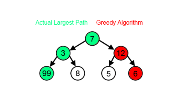
2. The Conditions for Applicability
So, the crucial question is: when can we trust a greedy algorithm? A problem must exhibit two specific properties for a greedy strategy to guarantee a globally optimal solution. These properties are the heart of this lesson.
Let's watch a concise overview of these two properties.
Let's return to the 'Greedy Algorithms Explained' video, which introduces the two key properties.
Watch the segment from 04:06 to 05:28. The video formally defines the 'Greedy Choice Property' and 'Optimal Substructure'.
Now, let's dive deep into each property.
A. The Greedy Choice Property
This property states that a globally optimal solution can be reached by making a locally optimal (greedy) choice. In other words, the best-looking choice at the current moment must be part of some globally optimal solution.
The classic example to illustrate this is the coin change problem.
- Case 1 (Greedy Works): If you need to make change for 48 cents using US coins (1, 5, 10, 25), the greedy approach is to take the largest coin possible at each step:
25 -> 10 -> 10 -> 1 -> 1 -> 1. This gives 6 coins, which is optimal. - Case 2 (Greedy Fails): If the available coins are {1, 3, 4} and you need to make change for 6 cents, the greedy approach would be
4 -> 1 -> 1(3 coins). However, the optimal solution is3 -> 3(2 coins).
In the second case, the greedy choice of taking a '4' was not part of the globally optimal solution. Therefore, the problem with that set of denominations does not have the greedy choice property.
For a more formal and rigorous look at this property, let's turn to a more advanced example: the Minimum Spanning Tree (MST) problem. Proving the greedy choice property for MST algorithms involves a powerful technique called a "cut and paste" argument.
12. Greedy Algorithms: Minimum Spanning Tree
This lecture from MIT OpenCourseWare on Greedy Algorithms provides an academic-level proof of the greedy choice property. Understanding the proof technique itself is a valuable skill.
Watch the segments from 28:34 to 32:16 and 32:46 to 40:37. The first part introduces a key lemma: the least-weight edge crossing any 'cut' of the graph must be in an MST. The second part provides the 'cut and paste' proof. Follow the logic of how an existing optimal solution is modified to include the greedy choice, proving that a greedy choice can lead to an optimal result.
The "cut and paste" argument is a standard way to prove greedy algorithms correct: assume an optimal solution doesn't use the greedy choice, then show you can "cut" a piece out and "paste" the greedy choice in to get an equally good or better solution.
B. Optimal Substructure
This property should feel familiar from our discussion on Divide and Conquer. It means that an optimal solution to the entire problem is composed of optimal solutions to its subproblems.
For a greedy algorithm, this means that after we make a greedy choice, the remaining problem is a smaller instance of the same problem. An optimal solution to this subproblem, combined with our greedy choice, must yield an optimal solution to the original problem.
Let's see how this is formally proven, again using the MST example.
12. Greedy Algorithms: Minimum Spanning Tree
Let's return to the MIT lecture. The instructor demonstrates the optimal substructure property in a very concrete way using 'edge contraction'.
Watch from 07:57 to 11:40 to understand how greedy algorithms relate to dynamic programming through optimal substructure. Then, watch the formal proof from 12:32 to 28:34. The key idea here is that if you make a correct greedy choice (picking an edge for the MST) and 'contract' that edge to simplify the graph, the optimal solution for the new, smaller graph can be combined with your original choice to solve the whole problem.
3. Case Study: The Knapsack Problem
The Knapsack Problem is a famous optimization problem that perfectly illustrates the subtleties of applying a greedy strategy. There are two main versions:
- Fractional Knapsack: You can take fractions of items.
- 0/1 Knapsack: You must take an entire item or leave it.
This distinction is critical. A greedy approach works for one but not the other.
This segment from the 'Greedy Algorithms Explained' video is an excellent practical demonstration. It explores different greedy criteria for the Fractional Knapsack problem and shows why the same logic fails for the 0/1 version.
Watch from 05:34 to 16:36. Pay close attention to: The different greedy criteria attempted (smallest size, largest value). The correct greedy criterion: highest value-to-size ratio. Why this exact same greedy strategy fails for the 0/1 Knapsack problem. This failure is a direct consequence of the problem not having the greedy choice property.
The reason the greedy strategy (highest value/weight ratio) works for the fractional knapsack is that the problem has both the greedy choice and optimal substructure properties. The resource below provides a formal proof.
PROVING GREEDY ALGORITHM GIVES THE OPTIMAL ...
This worksheet from UC Riverside walks through the formal proofs for the Fractional Knapsack problem, cementing the theory we've discussed.
Read the sections 'Introduction', 'Prove Greedy Choice Property', and 'Showing optimal substructure'. This will connect the abstract definitions of the properties to a concrete algorithmic proof.
The 0/1 Knapsack problem, on the other hand, lacks the greedy choice property. Taking the item with the best ratio might prevent you from taking two other items that, together, would have been more valuable. This is a classic case where a more powerful technique, like Dynamic Programming, is required.
Test your understanding!
You are a developer building a log processing system. You have a list of tasks, each with a start time and an end time. You want to run as many tasks as possible on a single machine, but no two tasks can overlap.
Consider these three greedy strategies:
- Always pick the task with the earliest start time.
- Always pick the task with the shortest duration.
- Always pick the task with the earliest end time.
Which of these strategies do you think will guarantee an optimal solution? Can you think of a counterexample for the strategies that won't work? (This is a famous problem called Activity Selection).
Show answer
The optimal strategy is #3: Always pick the task with the earliest end time.
Here are counterexamples for the other two:
-
Counterexample for #1 (Earliest Start Time):
- Task A: [0, 10]
- Task B: [1, 3]
- Task C: [4, 6]
Greedy choice picks Task A first because it starts earliest. After that, no other tasks can run. The optimal solution is to pick B and C (2 tasks).
-
Counterexample for #2 (Shortest Duration):
- Task A: [0, 4]
- Task B: [5, 9]
- Task C: [3, 6] (shortest duration)
Greedy choice picks Task C first. After that, no other tasks can run. The optimal solution is to pick A and B (2 tasks).
Strategy #3 (earliest end time) works because it maximizes the amount of time remaining for other activities. This is a classic greedy problem that we will implement in the next lesson.
Conclusion
In this lesson, we established a mental framework for the Greedy paradigm. You've moved beyond simply knowing what a greedy algorithm is to understanding the critical conditions that govern its success. This analytical ability to validate an algorithmic approach before implementation is a hallmark of a senior engineer's architectural thinking.
Key Takeaways:
- A Greedy Algorithm builds a solution by making a series of locally optimal choices.
- This approach is only guaranteed to be optimal if the problem exhibits two key properties:
- Greedy Choice Property: The locally optimal choice is always part of some globally optimal solution.
- Optimal Substructure: The optimal solution contains optimal solutions to its subproblems.
- Problems like Fractional Knapsack meet these criteria, while closely related problems like 0/1 Knapsack do not.
- Always be prepared to justify why a greedy approach is valid for a given problem, often by proving these two properties or by creating a counterexample if they don't hold.
Preview of the Next Lesson:
Now that we have a solid theoretical foundation, it's time to put it into practice. In our next lesson, we will apply a greedy algorithm to solve a classic optimization problem. We will focus on the implementation of the Activity Selection problem, paying close attention to how our choice of data structures and initial sorting step are critical to an efficient greedy solution.