DFS: Exploration and Connectivity

1. The Core Idea: Exploring a Labyrinth

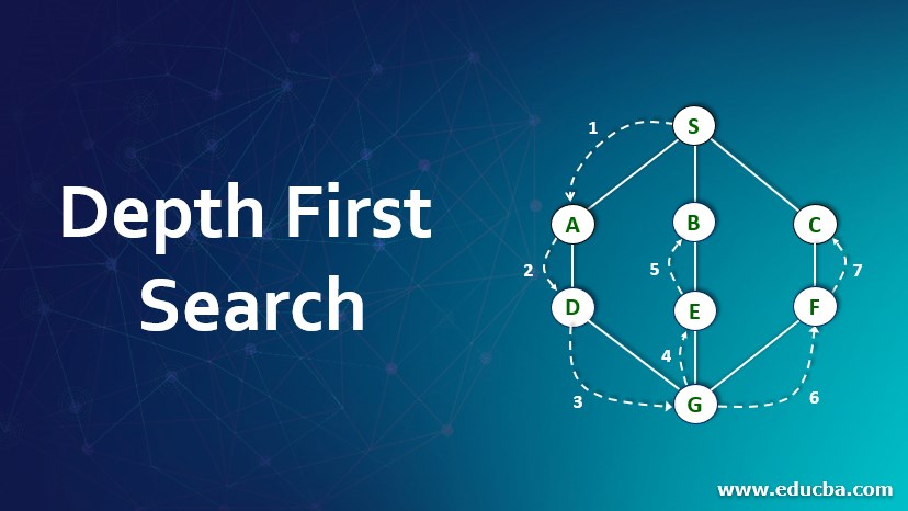
Imagine you're in a labyrinth and want to find the exit. One natural strategy is to pick a path and follow it as far as you can. If you hit a dead end, you backtrack to the last intersection where you had an unexplored path and try that one. You keep doing this, marking your path so you don't go in circles, until you find the exit or have explored every passage.

This is precisely the intuition behind Depth-First Search. It explores as far as possible along each branch before backtracking.

To get a feel for this process, let's watch a short, intuitive explanation.

The most critical takeaway from that demonstration is the need to mark vertices as "visited." Without this, if the graph contains a cycle (e.g., A -> B -> C -> A), the algorithm would loop forever.

2. Implementing Depth-First Search

DFS can be implemented in two primary ways: recursively (which is often more intuitive) and iteratively (which avoids potential recursion depth limits). Since you're interested in building a solid foundational understanding, we will cover both. For both implementations, we'll assume the graph is represented by an adjacency list, which you learned about in the previous lesson.

Recursive Implementation

The recursive approach is elegant because the program's call stack naturally handles the backtracking process. When a function calls itself for a neighbor, it goes "deeper." When that function returns, it automatically "backtracks" to the previous state.

Here is the logic in pseudocode, which captures the essence of the algorithm independent of any programming language:

function DFS(vertex, visited_set):
  mark vertex as visited
  // Process the vertex here (e.g., print it)
  
  for each neighbor in adjacency_list_of(vertex):
    if neighbor is not in visited_set:
      DFS(neighbor, visited_set)

To start the search on a graph G from a start_node, you would initialize an empty visited_set and call DFS(start_node, visited_set).

Iterative Implementation

The iterative approach achieves the same result but uses an explicit stack data structure instead of the implicit call stack. This can be more efficient in terms of memory management for very deep or skewed graphs and avoids stack overflow errors. Your knowledge of stacks from earlier in the course is directly applicable here.

The logic is as follows:

1. Initialize a stack and push the starting vertex onto it.
2. Initialize a visited set.
3. While the stack is not empty:
   a. Pop a vertex from the stack.
   b. If it hasn't been visited, mark it as visited and process it.
   c. Push all its unvisited neighbors onto the stack.

Here's the iterative pseudocode:

function DFS_iterative(start_node):
  create an empty stack
  push start_node onto stack
  create an empty visited_set

  while stack is not empty:
    vertex = pop from stack
    
    if vertex is not in visited_set:
      mark vertex as visited
      // Process the vertex here
      
      for each neighbor in adjacency_list_of(vertex):
        if neighbor is not in visited_set:
          push neighbor onto stack

To see these algorithms written out more formally, you can review the following resource.

3. Complexity Analysis

As you requested, let's integrate complexity analysis. Understanding the performance of DFS is crucial for making architectural decisions.

• Time Complexity: $O(V+E)$
  • V is the number of vertices, and E is the number of edges.
  • Each vertex is visited (pushed onto the stack/recursively called) exactly once, thanks to the visited set. This accounts for the $O(V)$ part.
  • When we are at a vertex, we iterate through its adjacency list. Over the entire run of the algorithm, each edge in the graph will be examined exactly once (for a directed graph) or twice (for an undirected graph). This accounts for the $O(E)$ part.
  • Therefore, the total time complexity is linear in the size of the graph representation, $O(V+E)$.

• Space Complexity: $O(V)$
  • The visited set will store up to V vertices in the worst case.
  • The stack (either the call stack for recursion or the explicit stack for iteration) will, in the worst case, hold up to V vertices. This happens in a graph that is a single long chain. The depth of recursion or the size of the stack would be V.
  • Thus, the space complexity is dominated by these factors, resulting in $O(V)$.

4. Applications of DFS

Now that you can implement and analyze DFS, let's explore what you can do with it. This is where the algorithm's power truly shines.

Pathfinding

Can we get from node A to node B? DFS can answer this easily. You start a DFS from node A and stop if you ever encounter node B. If the DFS completes without ever visiting node B, no path exists.

Connectivity

DFS is excellent for exploring the structure of a graph.

• Finding Connected Components: In an undirected graph, a "connected component" is a subgraph where every vertex is reachable from every other vertex. You can find all components by:
  1. Picking an arbitrary unvisited vertex.
  2. Running DFS from it. All vertices visited by this DFS form one component.
  3. If there are still unvisited vertices in the graph, repeat step 1.
• Cycle Detection: A simple modification to DFS can detect cycles. During a traversal, if you encounter an edge that points to a vertex that is already in the current recursion stack (not just 'visited', but actively being explored), you have found a back edge, which indicates a cycle. We will cover this in more detail in a future lesson.
• Topological Sorting: For a Directed Acyclic Graph (DAG), DFS can be used to produce a linear ordering of vertices such that for every directed edge from u to v, u comes before v in the ordering. This is critical for scheduling tasks with dependencies.

Conclusion

In this lesson, you have taken a deep dive into Depth-First Search, a cornerstone algorithm for graph traversal. You have moved from the high-level concept of "exploring a maze" to concrete recursive and iterative implementations, along with a formal analysis of their performance.

Key Takeaways:

• DFS explores deeply, following a path to its end before backtracking.
• It is implemented either recursively (using the call stack) or iteratively (using an explicit stack).
• A visited set is essential to prevent infinite loops and redundant work.
• The time complexity is $O(V+E)$, and space complexity is $O(V)$, making it efficient for most graphs.
• DFS is a versatile tool used for pathfinding, analyzing connectivity, detecting cycles, and more.

Preview of the Next Lesson:
DFS explores a graph by going deep. But what if we wanted to explore layer by layer, like ripples in a pond? In the next lesson, we will cover Breadth-First Search (BFS). You will learn how it uses a queue instead of a stack to achieve this "wide" traversal and discover its unique application in finding the shortest path in unweighted graphs.