BFS: Implementation & Shortest Path Applications

1. The Core Idea: Exploring Layer by Layer

Imagine you are at the center of a social network and want to find the connection path with the fewest "friend-of-a-friend" hops to another person. You wouldn't follow one long chain of connections. Instead, you'd check all your direct friends (level 1), then all their friends (level 2), and so on, until you find the person.

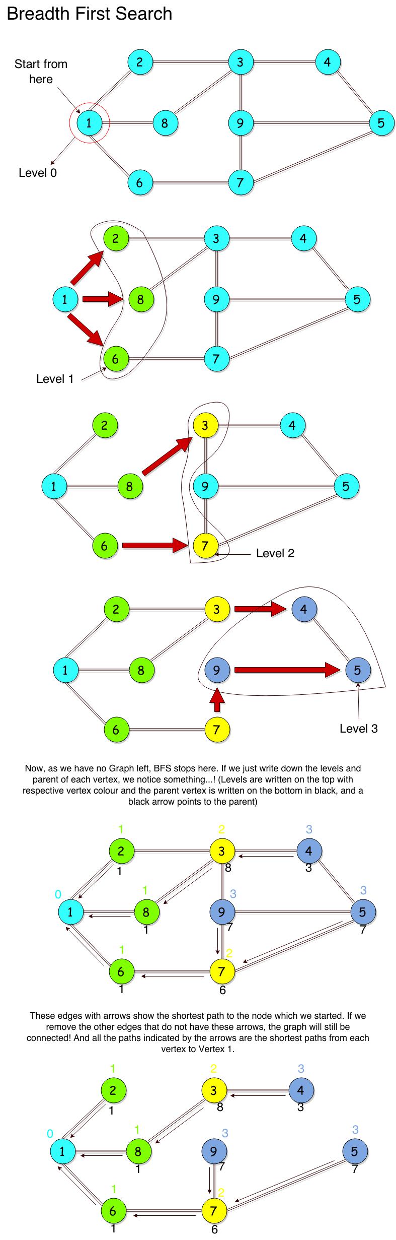
This is the exact intuition behind Breadth-First Search. It starts at a source node and explores all its immediate neighbors first, before moving on to the next level of neighbors.

The key to achieving this level-by-level exploration is using a Queue, which operates on a First-In, First-Out (FIFO) principle. This is the fundamental difference from DFS, which uses a Last-In, First-Out (LIFO) stack.

To see this in action, let's start with a video that visualizes the process.

As you saw, the queue ensures that we fully explore all nodes at a given distance (or "level") from the source before moving to nodes at the next level.

2. The BFS Algorithm and Complexity

The formal algorithm for BFS is quite straightforward and builds on concepts you're already familiar with from DFS, like the visited set.

The steps are:

1. Initialize a queue and add the start_node to it.
2. Initialize a visited set and add the start_node to it.
3. While the queue is not empty:
   a. Dequeue a node (let's call it current_node).
   b. Process current_node.
   c. For each neighbor of current_node:
   i. If the neighbor has not been visited:
   - Add it to the visited set.
   - Enqueue the neighbor.

Complexity Analysis

As noted in the article, the complexity of BFS is identical to DFS:

• Time Complexity: $O(V+E)$

  • Each vertex is enqueued and dequeued exactly once, which is $O(V)$.
  • Every edge is examined once (for directed graphs) or twice (for undirected graphs) when we check the neighbors of each vertex. This is $O(E)$.
  • The total time is therefore linear in the size of the graph.

• Space Complexity: $O(V)$

  • The visited set can store up to $V$ vertices.
  • The queue, in the worst-case scenario (a very wide, shallow graph), might need to hold nearly all the vertices at once. For instance, in a star graph, after visiting the center node, all $V-1$ other nodes are added to the queue. Therefore, the space complexity is $O(V)$.

3. Application: Shortest Path in Unweighted Graphs

Here is the most significant application of BFS. Because it explores level by level, BFS is guaranteed to find the shortest path from a source node to all other nodes in an unweighted graph. The "shortest path" here means the path with the minimum number of edges.

The first time BFS reaches a target node, it is guaranteed to be via a shortest path. Why? Because if a shorter path existed, BFS would have discovered the target node at an earlier level.

To implement this, we can modify our algorithm slightly. Instead of just a visited set, we'll use a distance array. This array will store the shortest distance from the source to every other node.

Let's watch a detailed walkthrough of this process.

Reconstructing the Path

Knowing the shortest distance is useful, but often you need the actual path. To do this, we need to track the "parent" of each node—that is, the node from which it was discovered. We can use a previous or parent array for this.

When BFS adds a neighbor to the queue, we record that the current_node is the parent of that neighbor. Once the BFS is complete (or the target is found), we can reconstruct the path by starting at the target node and backtracking through the parent pointers until we reach the source.

The following video segments explain this path reconstruction logic.

This combination of finding distances and then reconstructing the path is a powerful technique that forms the basis for more complex shortest path algorithms like Dijkstra's, which you'll encounter later.

4. Implementation in Practice

As a software engineer, translating this theory into code is the final step. The resources below provide a path from a basic Graph class to a full implementation of BFS for finding shortest paths.

The guide's approach of encapsulating graph logic within a class is a common and effective software engineering practice.

Conclusion

Today you've added another fundamental tool, Breadth-First Search, to your algorithmic toolkit. You've seen how a simple switch from a stack (DFS) to a queue (BFS) changes the entire exploration strategy from "deep" to "wide."

Key Takeaways:

• BFS explores level-by-level using a queue (FIFO) to maintain the order of nodes to visit.
• Its time complexity is $O(V+E)$ and space complexity is $O(V)$, just like DFS.
• The key application of BFS is finding the shortest path in unweighted graphs, a problem it solves optimally due to its layered traversal.
• Path reconstruction is done by tracking each node's parent during the traversal and backtracking from the target.

Preview of the Next Lesson:
We've now covered the two main ways to traverse a graph. In the next lesson, we will revisit DFS to see how we can augment it to solve another critical problem: detecting cycles in both directed and undirected graphs. This is a crucial capability for tasks like validating dependencies, finding deadlocks, and ensuring a graph has properties required for other algorithms (like topological sorting).