Graph Representations: Adjacency Matrices vs. Lists

1. What is a Graph?

At its core, a graph is simply a collection of vertices (or nodes) and edges that connect pairs of vertices. Unlike trees, graphs don't have a root or a strict parent-child hierarchy. Any node can be connected to any other node, and these connections can even form cycles.

To get a quick and practical introduction to graph terminology, please watch the beginning of the following video.

As you saw in the video, we primarily distinguish between:

• Undirected Graphs: Edges are two-way. If A is connected to B, B is also connected to A (like a Facebook friendship).
• Directed Graphs: Edges are one-way, represented by arrows. If A is connected to B, it doesn't mean B is connected to A (like a Twitter follow).

Now, how do we store this structure in a computer's memory? A drawing is intuitive for us, but a program needs a concrete data structure.

2. Adjacency Matrix

The first common representation is the adjacency matrix. It's a two-dimensional array (a matrix) of size $V\times V$, where $V$ is the number of vertices. We typically label our vertices from 0 to $V-1$.

The rule is simple:

• matrix[i][j] = 1 if there is an edge from vertex i to vertex j.
• matrix[i][j] = 0 if there is no edge.

For a weighted graph, we can store the edge weight instead of 1. For an undirected graph, the matrix will be symmetric (matrix[i][j] == matrix[j][i]).

Analysis of Adjacency Matrix

• Space Complexity: It always requires $O(V^2)$ space, regardless of the number of edges. This is because we must allocate memory for every possible pair of vertices.
• Time Complexity of Operations:
  • Check for an edge (u, v): O(1). This is its greatest strength. We just look up matrix[u][v].
  • Add/remove an edge (u, v): O(1). We just set the value at matrix[u][v].
  • Find all neighbors of a vertex u: O(V). We must iterate through the entire row matrix[u] to see which columns have a 1.

3. Adjacency List

The second major representation is the adjacency list. Instead of a matrix, we use an array (or a hash map) where each entry corresponds to a vertex. Each entry stores a list (like a linked list or dynamic array) of that vertex's neighbors.

• adjList[i] contains a list of all vertices j such that there is an edge from i to j.

Given your background, you can think of this as an object or map where keys are vertex IDs and values are arrays of their neighbors.

The image above also shows an example of an adjacency list on the right.

Analysis of Adjacency List

• Space Complexity: It requires $O(V+E)$ space, where E is the number of edges. We need V space for the main array/map and then space proportional to the number of edges to store all the neighbor lists. For an undirected graph, each edge appears twice, so it's $O(V+2E)$, which is still $O(V+E)$.
• Time Complexity of Operations:
  • Check for an edge (u, v): O(degree(u)), where degree(u) is the number of neighbors of u. In the worst case, this is O(V). We have to scan the neighbor list of u to see if v is in it.
  • Add an edge (u, v): O(1). We just append v to the list at adjList[u].
  • Find all neighbors of a vertex u: O(degree(u)). This is very efficient as we can just retrieve the list directly.

4. Trade-offs and When to Use Each

The choice between an adjacency matrix and an adjacency list is a classic space-time trade-off that depends on the characteristics of the graph.

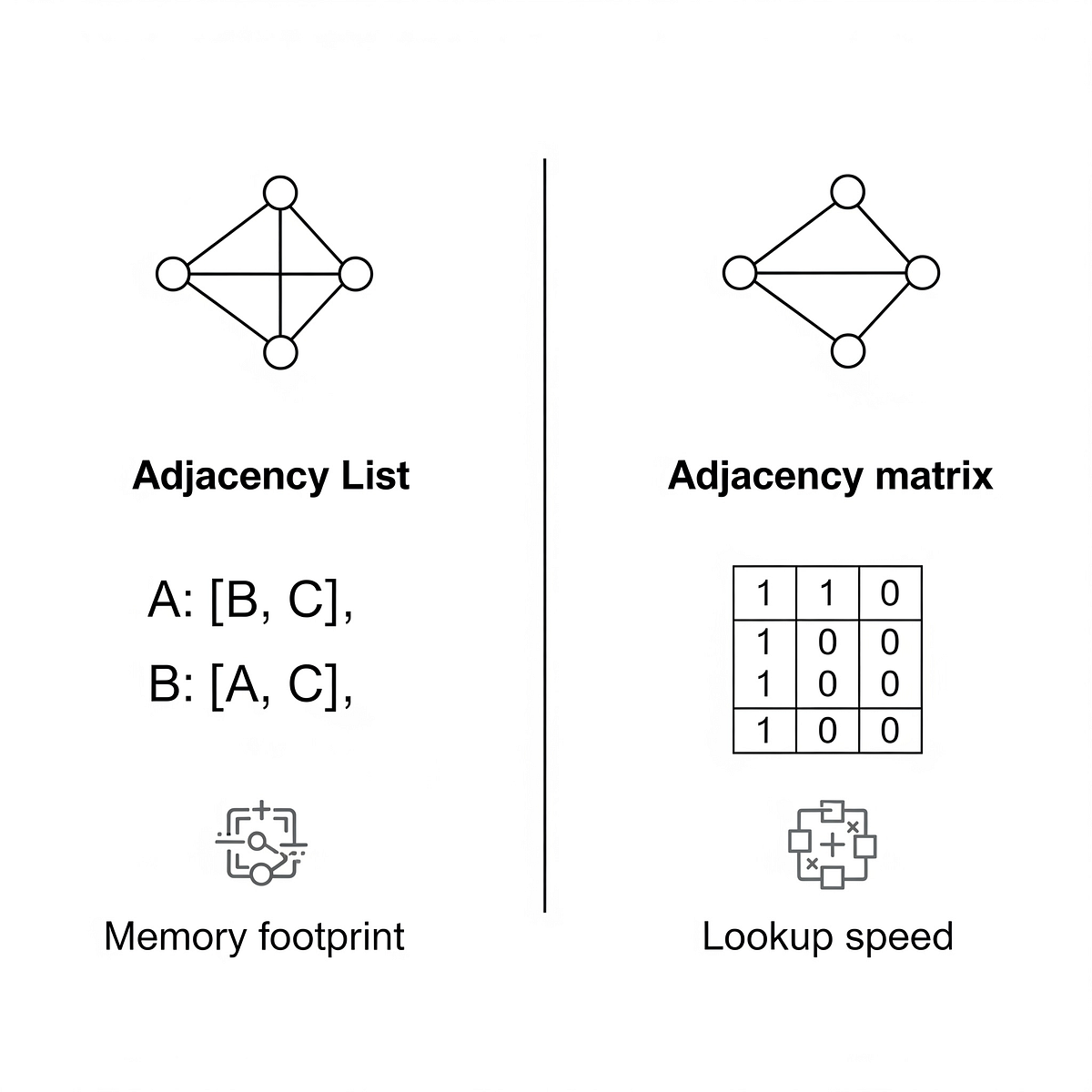
The key factor is the density of the graph.

• A dense graph is one where the number of edges E is close to the maximum possible, $V^2$. In this case, the $O(V^2)$ space of an adjacency matrix is acceptable, and its fast O(1) edge lookup is a significant advantage.
• A sparse graph is one where the number of edges E is much smaller than $V^2$ (e.g., closer to V). Most real-world graphs, like social networks and road systems, are sparse. For these, the $O(V+E)$ space of an adjacency list is far more efficient.

To formalize this analysis and see how these representations translate into a more formal API, the following document from Carnegie Mellon University is a great resource.

Because most real-world graphs are sparse, the adjacency list is the most common representation used in practice. Its efficiency in storing and retrieving neighbors is crucial for the graph traversal algorithms we will study next.

Conclusion

You've now learned the two primary methods for representing graphs and the critical factors that guide the choice between them. This is a fundamental concept that underpins all graph algorithms.

Key Takeaways:

• Graphs model networks of vertices and edges. They can be directed or undirected.
• An Adjacency Matrix is a $V\times V$ matrix with O(1) edge lookup but requires $O(V^2)$ space, making it suitable for dense graphs.
• An Adjacency List is an array of neighbor lists with O(degree(v)) neighbor lookup and requires $O(V+E)$ space, making it ideal for sparse graphs.
• The choice of representation is an architectural decision based on graph density and the most frequent operations you need to perform. For most common applications, the adjacency list is preferred.

Preview of the Next Lesson:
Now that we know how to store a graph, we can start exploring it. In the next lesson, we will learn our first major graph traversal algorithm: Depth-First Search (DFS). You will learn how to implement it and see its applications in solving problems like finding a path between two nodes and checking for connectivity.