Hello! Welcome to the first lesson in our new module, "Hashing, Trees, and Search."
In the last module, we concluded by examining space complexity and the critical trade-offs between time, memory, and design choices. We saw that no single solution is perfect for all scenarios; engineering is about choosing the right tool for the job.
Today, we dive into one of the most widely used data structures in all of computer science: the hash table (often called a hash map or dictionary in various programming languages). Hash tables are a masterful example of a time-space trade-off. They are designed to achieve an average time complexity of for lookups, insertions, and deletions—a remarkable feat.
Our goal in this lesson is to understand the fundamental mechanics that make this possible. We will explore what a hash function is, why "collisions" are an unavoidable consequence of its use, and the primary strategies for resolving them. Understanding these concepts is essential not just for using hash tables effectively, but for making informed architectural decisions when designing systems that require high-performance data access.
1. The Goal: Searching in Constant Time
Before diving into the mechanics, let's understand the problem hash tables are designed to solve.
Hashing Technique - Simplified
The video 'Hashing Technique - Simplified' by Abdul Bari provides an excellent motivation for why we need hashing in the first place, contrasting it with slower search methods.
Watch the first 2 minutes of the video (00:00 to 02:08). Focus on the progression from linear search (O(n)) to binary search (O(\log n)) and the ultimate goal of achieving constant time (O(1)) lookups.
As the video explains, the core idea is to find a way to compute the storage location of an item directly from the item's key, rather than searching for it. This computation is the job of a hash function.
2. The Hash Function
A hash function is a procedure that takes a key as input and returns an integer, known as a hash code. This hash code is then mapped to an index in an array, where the corresponding value is stored.
For a hash function to be effective, it needs several key properties.
The article 'Hash Map Deep Dive' explains the properties of a good hash function. This is critical for understanding why some hash tables perform better than others.
Read the section titled 'What Is a Hash Function?'. Pay close attention to the four properties listed: Deterministic, Uniform Distribution, Fast Computation, and Minimize Collisions.
In summary, a good hash function should:
- Be deterministic: The same key must always produce the same hash code.
- Distribute keys uniformly: It should spread keys evenly across the array slots to avoid clustering everything in a few spots.
- Be fast: The hash calculation itself should not become a performance bottleneck.
- Minimize collisions: While impossible to eliminate, it should reduce the probability that two different keys produce the same hash code.
The simplest hash function, and a common starting point, is the modulo operator: index = hash(key) % table_size.
3. The Inevitable Problem: Collisions
Imagine we have a hash table of size 10 and we want to insert the key 23. Using the simple hash function key % 10, the index is 3. Now, what if we want to insert key 33? The index is also 3. This is a collision: two different keys have mapped to the same index.
Because the universe of possible keys (e.g., all possible strings) is virtually infinite, but the hash table size is finite, the Pigeonhole Principle guarantees that collisions are inevitable. Therefore, the strategy we choose to handle these collisions is the most important design decision in a hash table.
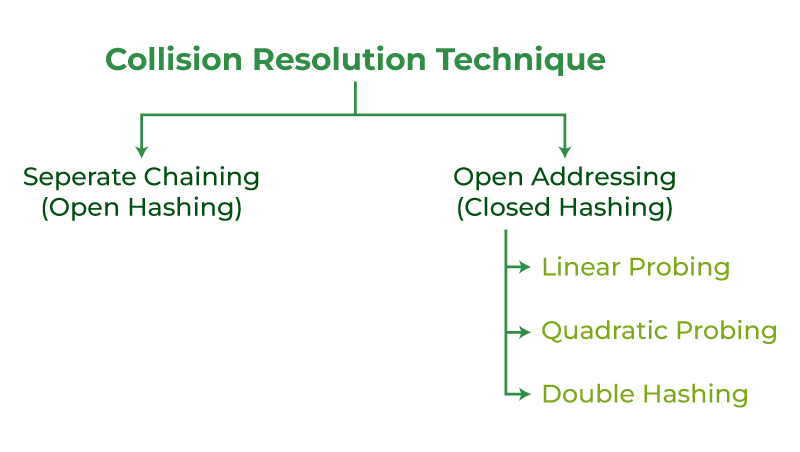
We'll now explore these two approaches in detail.
4. Collision Resolution Strategy 1: Separate Chaining
The most straightforward way to handle collisions is to make each slot in the hash table an independent container, most commonly a linked list. This method is called separate chaining.
When a key-value pair is inserted, we compute its hash index. Then, we simply add the new pair to the linked list at that index.

To understand the mechanics and trade-offs, let's watch a detailed explanation.
Collision Handling in Hash Tables
The video 'Collision Handling in Hash Tables' by Mary Elaine Califf provides a clear, visual walkthrough of how separate chaining works for insertion, search, and deletion.
Watch from the beginning to 02:54. Observe how new elements are typically added to the front of the list for efficiency and how searching requires traversing the list at the target index.
Trade-offs of Separate Chaining:
- Pros:
- Simple to implement: The logic for insertion and deletion is straightforward linked list manipulation.
- Handles high load factors well: The performance degrades smoothly as the table fills up. The number of elements can even exceed the table size.
- Cons:
- Memory overhead: Every entry requires extra memory for the linked list pointers.
- Poor cache performance: Linked list nodes can be stored far apart in memory. When you traverse a list, the CPU may have to fetch data from different parts of main memory, which is slow compared to accessing a contiguous block of an array.
Test your understanding!
Given an empty hash table of size 7 and a hash function h(k) = k % 7, show the state of the table after inserting the keys {10, 2, 16, 9, 23} using separate chaining.
Show answer
The insertions would proceed as follows:
10 % 7 = 3. Insert 10 at index 3.2 % 7 = 2. Insert 2 at index 2.16 % 7 = 2. Collision! Add 16 to the list at index 2.9 % 7 = 2. Collision! Add 9 to the list at index 2.23 % 7 = 2. Collision! Add 23 to the list at index 2.
The final table would look like this (assuming new elements are added to the front of the list):
- Index 0:
null - Index 1:
null - Index 2:
-> 23 -> 9 -> 16 -> 2 - Index 3:
-> 10 - Index 4:
null - Index 5:
null - Index 6:
null
5. Collision Resolution Strategy 2: Open Addressing
Open addressing takes a different approach: all key-value pairs are stored directly inside the main array. If a collision occurs at index i, the algorithm probes (checks) for another open slot in the table according to a fixed sequence.
There are several common probing strategies. Let's review them using the same video.
Collision Handling in Hash Tables
Continuing with 'Collision Handling in Hash Tables', we will now explore the three main types of open addressing: linear probing, quadratic probing, and double hashing.
Watch from 02:54 to 16:28. For each technique, focus on: Linear Probing (02:54): How it works and what 'primary clustering' is. Quadratic Probing (07:47): How its probe sequence differs and how it reduces clustering. Double Hashing (12:14): How it uses a second hash function to create unique probe sequences.
Let's summarize these techniques.
a. Linear Probing
This is the simplest strategy. If index h(k) is occupied, we try h(k) + 1, then h(k) + 2, and so on, wrapping around the table if necessary.
- Problem: Primary Clustering. As the table fills, long blocks of occupied cells emerge. When a key hashes into this block, it must traverse to the end of the block, making the block even longer for the next collision. This leads to a rapid decline in performance.
b. Quadratic Probing
To avoid primary clustering, quadratic probing uses a probe sequence that jumps by quadratically increasing amounts: h(k) + 1^2, h(k) + 2^2, h(k) + 3^2, etc.
- Improvement: Keys that hash to the same area are more likely to find an empty slot quickly, as they jump farther away on subsequent probes.
- Problem: Secondary Clustering. If two keys have the same initial hash index, they will follow the exact same probe sequence, which is an inefficiency.
c. Double Hashing
This is the most sophisticated of the three methods. It uses a second hash function, h2(k), to determine the step size for the probe sequence: (h1(k) + i * h2(k)) % table_size.
- Improvement: Keys that hash to the same initial location will almost certainly have different second hash values, and thus follow different probe sequences. This effectively eliminates clustering and gives the best performance among open addressing techniques.
Deletion in Open Addressing: The Tombstone Problem
A critical issue arises in open addressing when you want to delete an element. If you simply empty the slot, you might break a probe chain for another element. For example, if you inserted keys A, B, and C, where A and B collided and B was placed after A, deleting A could make C unreachable if its probe sequence went through A's original slot.
The solution is logical deletion. Instead of emptying the slot, we mark it with a special "tombstone" value. This tells the search algorithm to keep probing, but tells the insert algorithm that the slot can be overwritten. The video Collision Handling in Hash Tables discusses this from 05:14 to 06:10.
6. Comparing the Strategies
Choosing a collision resolution strategy involves significant architectural trade-offs between memory, cache performance, and complexity. For your work as an engineer, having a clear summary of these trade-offs is invaluable.
The article 'Hash Map Deep Dive' contains an excellent summary table comparing all the collision resolution methods we've discussed.
First, read the text descriptions under 'Collision Resolution'. Then, carefully study the summary table that compares Chaining, Linear Probing, Quadratic Probing, and Double Hashing across various factors like complexity, clustering, and memory overhead.
Here is a simplified version of that comparison:
| Feature | Separate Chaining | Linear Probing | Quadratic Probing | Double Hashing |
|---|---|---|---|---|
| Space Efficiency | Lower (pointers) | Highest | High | High |
| Cache Performance | Poor (scattered lists) | Excellent (sequential access) | Good | Moderate |
| Clustering Issue | None | Primary (severe) | Secondary (mild) | Minimal |
| Deletion | Simple | Complex (tombstones) | Complex (tombstones) | Complex (tombstones) |
| Implementation | Simple | Simple | Moderate | Complex |
This table highlights the core trade-off: Separate Chaining uses more memory and has worse cache performance but is simple and robust. Open Addressing, especially linear probing, is highly cache-friendly but suffers from clustering and complex deletions.
Conclusion
In this lesson, you have learned the theoretical underpinnings of hash tables, one of the most important data structures for a software engineer.
Key Takeaways:
- A hash function maps a key to an array index, aiming for access time.
- Collisions are unavoidable and must be resolved with a deliberate strategy.
- Separate Chaining resolves collisions by storing colliding elements in a linked list at the hashed index. It is simple and robust but less memory- and cache-efficient.
- Open Addressing resolves collisions by probing for the next empty slot within the table array itself. It is cache-friendly but suffers from clustering and requires tombstones for deletion.
- Different open addressing techniques (Linear Probing, Quadratic Probing, Double Hashing) offer different trade-offs in mitigating clustering at the cost of increased complexity.
With this theoretical foundation, you are now ready for the practical part. In our next lesson, you will implement a hash table from scratch, putting these concepts of hashing, collision resolution, and their trade-offs into practice.