Hello! Welcome to the final lesson in our "Data Structures & Algorithmic Analysis" module.
In our previous lessons, we've devoted significant attention to analyzing the time complexity of algorithms—how their runtime scales with input size. This is a crucial metric, but it's only half the story. As you move towards an architectural mindset, you'll find that making sound design decisions requires balancing multiple constraints, and one of the most important is memory.
Today, we'll address the other side of the performance coin: space complexity. Our goal is to formalize how we measure an algorithm's memory usage and, more importantly, to analyze the trade-offs between space, time, and design choices. This skill is essential for building scalable and efficient systems, especially when dealing with large datasets or resource-constrained environments.
1. Defining Space Complexity
At its core, space complexity is a measure of the total memory an algorithm needs to run, expressed as a function of the input size. When analyzing this, we typically break memory usage into two categories.

- Input Space: The memory used to store the input data itself. For an algorithm that processes an array of size
n, the input space is . - Auxiliary Space: The extra or temporary memory an algorithm uses during its execution. This includes variables, data structures, and the memory used by function calls (the call stack).
In most contexts, when software engineers discuss the "space complexity" of an algorithm, they are referring to the auxiliary space complexity. This is because we want to measure the memory cost of the algorithm's logic, separate from the memory needed just to hold the input.
Like time complexity, space complexity is described using Big-O notation.
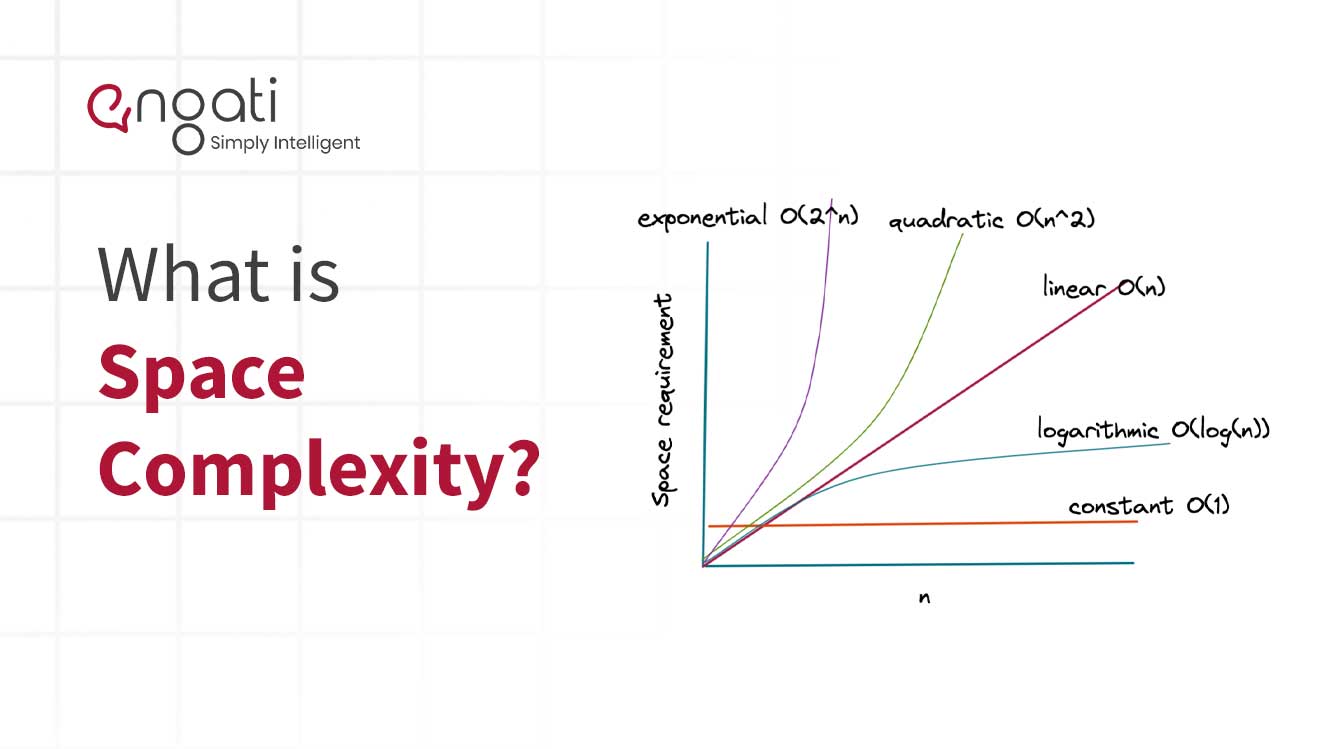
Let's begin by reading a short article that defines these concepts and provides a few clear, initial examples.
Understanding Space Complexity and How to Analyze It
The article 'Understanding Space Complexity and How to Analyze It' by Noor Fatima provides a clear definition of space complexity and shows simple examples of constant and linear space usage.
Read the sections 'What is Space Complexity?', 'Analyzing Space Complexity Step-by-Step', and the first three 'Examples of Space Complexity' (Constant, Linear, and Recursive Function). Focus on how the memory usage relates to the input size n in each case.
As the article demonstrates:
- or Constant Space: The algorithm uses a fixed amount of memory regardless of the input size. Simple arithmetic operations or swapping two variables are good examples.
- or Linear Space: The memory usage grows proportionally to the input size. Creating a copy of an input array is a classic example.
2. The Hidden Cost of Recursion: The Call Stack
One of the most common sources of auxiliary space usage, and one that is easy to overlook, is the call stack. When a function calls another function, the system saves the state of the caller (its local variables and where it left off) in a block of memory called a stack frame. In a recursive algorithm, a new stack frame is created for every pending recursive call.
The maximum number of stack frames on the call stack at any one time determines the space complexity of the recursion. Let's watch a video that visualizes this process for the factorial function.
Time and space complexity analysis of recursive programs - using factorial
The video 'Time and space complexity analysis of recursive programs' from mycodeschool provides an excellent visualization of how the call stack consumes memory during a recursive call.
Watch from 03:22 to 08:01. Observe how each call to Factorial(n) adds a new frame to the memory stack. Pay close attention to how the stack grows to its maximum depth and then shrinks as the functions return.
The video clearly shows that for an input n, the recursion depth is n. Therefore, the space complexity of the recursive factorial is .
Now, let's solidify this concept by reading a detailed analysis of recursion, which also clarifies a common misconception about more complex recursive functions like Fibonacci.
Time and Space Complexity for Recursive Algorithms
The article 'Time and Space Complexity for Recursive Algorithms' from Launch School explains how to analyze space by focusing on the maximum depth of the call stack.
Read from the beginning of the 'Space Complexity' section to the end of the article. First, understand the analysis for the Factorial algorithm. Then, pay close attention to the step-by-step breakdown for the Fibonacci algorithm. Note why its space complexity is O(n) (proportional to its depth) and not O(2^n) (proportional to the total number of calls).
The key takeaway is that space complexity for recursion is determined by the maximum depth of the recursion tree, not the total number of nodes in the tree. Even though the recursive Fibonacci function makes an exponential number of calls, the call stack only ever grows to a depth of n.
Test your understanding!
Consider this simple recursive function to sum the elements of an array:
int recursiveSum(int[] arr, int n) {
    if (n <= 0) {
        return 0;
    }
    return recursiveSum(arr, n - 1) + arr[n - 1];
}
What is the auxiliary space complexity of this function, and why?
Show answer
The auxiliary space complexity is .
Each recursive call to recursiveSum adds a new frame to the call stack. The function calls itself with n-1, n-2, and so on, until it reaches the base case n=0. At its deepest point, there will be n pending function calls on the stack. Therefore, the memory usage is proportional to the input size n.
3. Identifying Memory Trade-offs
Analyzing space complexity isn't just an academic exercise. It's about making informed engineering decisions. Often, you will face a trade-off between time and space.
Trade-off 1: In-place vs. Out-of-place Algorithms
An in-place algorithm transforms the input data using a very small, constant amount of extra memory ( auxiliary space). An out-of-place algorithm requires additional memory, often proportional to the input size, to hold temporary data.
Sorting algorithms provide a perfect illustration of this trade-off. Let's see how.
Sorting Algorithms Time and Space Complexity | Sorting Algorithms | Big-O | Geekific
The video 'Sorting Algorithms Time and Space Complexity' by Geekific compares the space usage of several common sorting algorithms.
Watch from 03:54 to 04:19 and then from 12:12 to the end (13:37). Pay attention to the distinction between: In-place sorts like Bubble Sort (O(1) space). Out-of-place sorts like Merge Sort (O(n) space for the temporary array). The special case of Quicksort, which is in-place but uses O(\log n) stack space for recursion.
Here's a summary of the trade-offs discussed:
| Algorithm | Time Complexity (Avg) | Auxiliary Space Complexity | Trade-off |
|---|---|---|---|
| Bubble/Insertion Sort | Very space-efficient, but slow for large inputs. | ||
| Merge Sort | Fast and stable, but at the cost of significant memory usage. | ||
| Quicksort | Fast on average and highly space-efficient due to its in-place partitioning and logarithmic stack depth. A great general-purpose choice. |
Trade-off 2: Iteration vs. Recursion
As we saw with the factorial function, a recursive solution can sometimes be more intuitive or easier to write, but it comes at the cost of stack space. An iterative solution to the same problem can often achieve the same result with auxiliary space.
Recursive Factorial ( space):
def factorial_recursive(n):
    if n == 0:
        return 1
    return n * factorial_recursive(n - 1)
Iterative Factorial ( space):
def factorial_iterative(n):
    result = 1
    for i in range(1, n + 1):
        result *= i
    return result
Choosing between them is an architectural decision. Is the clarity of recursion worth the extra memory cost? For small n or shallow recursion, it might be. For deep recursion or in memory-constrained systems, the iterative approach is superior.
Trade-off 3: Data Structure Choice
The data structure you choose to represent your data has a profound impact on space (and time) complexity. We will see this in detail in the next module, but let's preview a classic example: representing a graph (like a social network).
- Adjacency Matrix: A 2D array of size (where is the number of vertices), where
matrix[i][j] = 1if there is an edge from vertexitoj.- Space Complexity:
- Time to check for an edge:
- Adjacency List: An array of lists, where
list[i]contains all the vertices adjacent to vertexi.- Space Complexity: (where is the number of edges)
- Time to check for an edge: , which is in the worst case.
The Trade-off:
If you are modeling a dense graph (where E is close to , e.g., every airport has flights to almost every other airport), the Adjacency Matrix is space-efficient and very fast for lookups.
However, if you are modeling a sparse graph (where E is much smaller than , e.g., a social network where a user is connected to a tiny fraction of all other users), the Adjacency Matrix would be mostly zeros and waste an enormous amount of space. The Adjacency List is far more memory-efficient in this common scenario.
Test your understanding!
You are tasked with designing a system to store the entire web as a graph for a search engine, where web pages are vertices and hyperlinks are edges. The web has billions of pages, but the average page links to only a few dozen other pages.
Considering space complexity as a critical constraint, would you recommend an Adjacency Matrix or an Adjacency List to represent this graph? Justify your answer.
Show answer
An Adjacency List is the only practical choice.
The web is a classic example of a massive but extremely sparse graph. The number of vertices is in the billions. If we used an Adjacency Matrix, the space required would be , which is astronomically large (billions squared) and completely infeasible to store.
With an Adjacency List, the space is . Since the average number of links per page (the average degree) is small, the number of edges is a small multiple of . The space is manageable, whereas is not. This is a clear case where choosing the right data structure based on space complexity analysis is paramount.
Conclusion
This lesson concludes our foundational module on data structures and algorithmic analysis. You've now seen that evaluating an algorithm requires a two-dimensional perspective, considering both time and space.
Key Takeaways:
- Space Complexity measures an algorithm's memory usage, typically focusing on auxiliary space (extra memory beyond the inputs).
- The call stack is a significant source of auxiliary space in recursive algorithms, with its size determined by the maximum recursion depth.
- Algorithm design is a game of trade-offs. You will constantly balance time vs. space, readability vs. performance (iteration vs. recursion), and choose data structures that fit the problem's constraints (in-place vs. out-of-place).
Next Steps
You've built a solid foundation with linear data structures (arrays, linked lists, stacks, queues) and the core principles of complexity analysis. In the next module, "Hashing, Trees, and Search," we will explore non-linear data structures that unlock more powerful and efficient ways to solve problems. We will begin by diving into hash tables, a data structure that offers remarkable average-case performance for lookups, insertions, and deletions.