Hash Table with Collision Resolution

Hello! Welcome back.

In our last lesson, we built a strong theoretical foundation for hash tables. We explored what a hash function is, why collisions are inevitable, and the two major strategies for resolving them: Separate Chaining and Open Addressing.

Today, we transition from theory to practice. Your goal for this lesson is to implement a hash table with collision resolution to support efficient lookups, insertions, and deletions. As a software engineer, translating abstract concepts into working code is the ultimate test of understanding. We will analyze complete implementations for both separate chaining and open addressing to see how their theoretical trade-offs manifest in actual code.

This practical approach will be crucial for developing the "architectural mindset" you're aiming for, allowing you to not just use a hash table, but to reason about its internal design and performance implications.

1. Implementing a Hash Table with Separate Chaining

Let's start with separate chaining, the strategy where each bucket in our table is a container (like a linked list or dynamic array) that holds all entries hashing to that index.

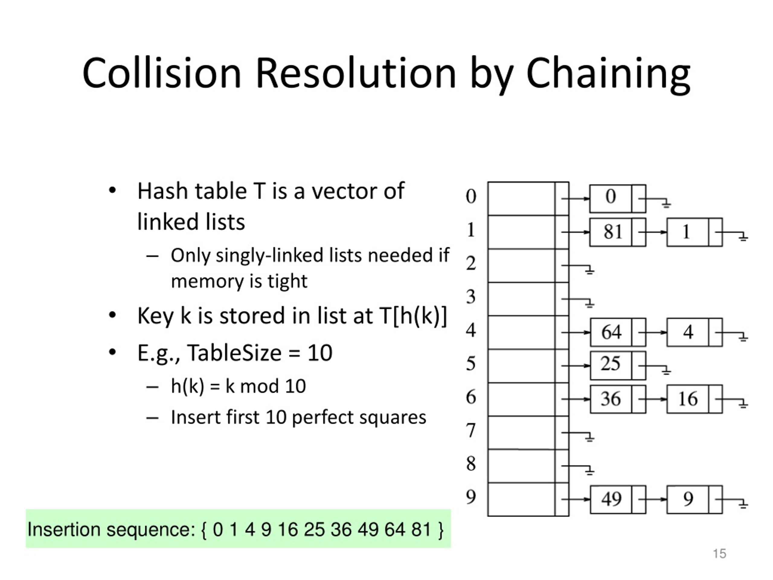
Collision Resolution by Chaining Example — Caption: A quick refresher from our last lesson. In separate chaining, keys that collide (like 16 and 36, which both hash to index 6) are stored in a list at that index.

The core of a separate chaining implementation involves an array of these lists and the logic to manage them during insert, get, and delete operations.

Hash Tables Demystified: A Complete Guide with PHP Implementation

The article 'Hash Tables Demystified' provides a complete, well-documented PHP implementation of a hash table using separate chaining. While the language is PHP, the object-oriented structure and logic are universal and easily translatable to other languages you know.

Read the section titled 'Complete PHP Implementation' and focus on the first code block, the HashTable class. Analyze the implementation of these key methods: __construct(): How the initial array of empty buckets is created. hash(): The function that converts a key into a bucket index. put(): Notice the two main steps: first, it checks if resizing is needed, then it finds the correct bucket and iterates through it to either update an existing key or append a new one. get(): How it finds the bucket and searches within the list for the specific key. remove(): How it finds the entry and splices it out of the bucket's array. resize(): This is a critical one. Observe how it creates a new, larger array of buckets and then re-hashes every single element from the old table into the new one.

Dissecting the Separate Chaining Implementation

Let's break down the logic from the PHP example:

Structure: The HashTable class uses a main array called $buckets. Each element of $buckets is itself an array, acting as the "chain" for that index.
Insertion (put):
1. The key is hashed to find an index, e.g., index = hash(key).
2. The code iterates through the chain at buckets[index].
3. If the key already exists in the chain, its value is updated. This prevents duplicate keys.
4. If the key is not found after checking the whole chain, the new key-value pair is appended to the end of the chain.
5. Crucially, it increments the total size and checks if the load factor (size / capacity) has exceeded a threshold. If so, it triggers a resize.
Deletion (remove):
1. The key is hashed to find the correct chain.
2. The code iterates through the chain to find the key-value pair.
3. Once found, the element is removed from the chain (e.g., using array_splice in PHP, or standard list removal in other languages).
4. The total size is decremented.

To see this logic explained in a different context, the following video implements the same ideas in C++.

C++ Hash Table Implementation

The video 'C++ Hash Table Implementation' provides a great walkthrough of the same logic. Watching this will help solidify the concepts in a different language.

Watch the sections covering the insert function (06:11 - 08:58) and the remove function (08:58 - 11:00). Compare the logic here with the PHP code you just reviewed. The core steps are identical: hash, find the list, iterate, and then either update/append or erase.

2. Implementing a Hash Table with Open Addressing

Now, let's turn to open addressing. Here, all entries are stored in the main array. When a collision occurs, we probe for the next available slot. We will focus on linear probing, the simplest probing strategy.

A key challenge in open addressing is deletion. As we discussed, simply clearing a slot can break a probe chain. The solution is to use tombstones—special markers indicating a slot is deleted but was once occupied.

Hash Tables Demystified: A Complete Guide with PHP Implementation

Let's return to the 'Hash Tables Demystified' article. It also provides an excellent implementation of a hash table using open addressing with linear probing.

Now, study the second code block, the HashTableOpenAddressing class. Pay close attention to the differences from the chaining implementation: Structure: Notice the use of three parallel arrays: $keys, $values, and $deleted (for tombstones). put(): Follow the while loop. It probes sequentially until it finds either (a) the same key to update, (b) a null or tombstoned slot to insert into, or (c) it loops back to the start (table is full). get(): The probe loop here is critical. It must continue probing past tombstones because the key it's looking for might be further down the probe chain. remove(): This method doesn't actually remove data. It finds the key and sets its corresponding flag in the $deleted array to true, creating a tombstone.

Dissecting the Open Addressing Implementation

The logic for open addressing is fundamentally different:

Structure: Instead of an array of lists, we have one flat array (or parallel arrays for keys and values). The state of each slot can be: empty (null), occupied, or a tombstone.
Insertion (put):
1. Hash the key to get a starting index.
2. Begin a probing loop.
3. If the current slot contains the same key, update the value and stop.
4. If the current slot is empty (null) or a tombstone, insert the new key-value pair there and stop.
5. If the slot is occupied by a different key, continue probing to the next slot ((index + 1) % capacity).
Deletion (remove):
1. Probe in the same way as get to locate the key.
2. Once found, instead of clearing the data, set a tombstone marker for that index. This ensures that future searches for other keys can correctly probe past this spot.
Search (get):
1. Hash the key to get a starting index.
2. Begin a probing loop.
3. If the slot contains the target key (and is not a tombstone), return its value.
4. If the slot is empty (null), the key does not exist in the table, so stop and return null.
5. If the slot is occupied by a different key or is a tombstone, continue probing.

Test your understanding!

In the open addressing implementation, the get method continues probing if it encounters a tombstone. What would happen if you modified the get method to stop and return null as soon as it hit a tombstone? Provide a short sequence of operations that would fail.

Show answer

This change would break the logic. A search for an item might fail even if the item is in the table.

Consider this sequence with a table of size 10 and hash function h(k) = k % 10:

put(12, "A"): Hashes to index 2. table[2] = {key: 12, value: "A"}.
put(22, "B"): Hashes to index 2 (collision). Linear probing places it at index 3. table[3] = {key: 22, value: "B"}.
remove(12): The entry at index 2 is marked with a tombstone.

Now, let's try to find key 22:

get(22): Hashes to index 2.
The get method checks table[2]. It finds a tombstone.
If the incorrect logic is used, it would stop here and return null, incorrectly reporting that key 22 is not in the table.

The correct logic must continue probing past the tombstone at index 2, find key 22 at index 3, and return its value "B".

3. Implementation Trade-offs Revisited

Having reviewed the code for both strategies, the theoretical trade-offs we discussed in the last lesson should now be much more concrete.

Factor	Separate Chaining	Open Addressing (Linear Probing)
Data Structure	Array of lists/arrays. Requires pointers/references, leading to scattered memory locations.	Flat arrays. Data is in a contiguous memory block.
Cache Performance	Potentially poor. Traversing a chain can cause cache misses.	Excellent. Linear probing accesses adjacent memory, which is very cache-friendly.
Deletion Logic	Simple: find the node in the list and remove it.	Complex: requires tombstones to maintain probe chains, adding state and complexity to `get` and `put`.
Memory Usage	Higher overhead due to pointers/references for each chain node.	More compact. No per-node overhead, but might have unused slots.

From an architectural standpoint, this is a classic space-time trade-off that also involves cache performance. Open addressing is often faster in practice for low-to-moderate load factors due to its superior cache locality, but its performance degrades sharply as the table fills, and the logic is more complex. Separate chaining is simpler to implement and degrades more gracefully, making it a robust, general-purpose choice.

Conclusion

In this lesson, you have successfully moved from theory to practice by analyzing the implementation of a hash table.

Key Takeaways:

Separate Chaining Implementation: Involves managing an array of lists. put, get, and remove operations require finding the correct list and then iterating through it. Deletion is a straightforward list-node removal.
Open Addressing Implementation: Involves probing for empty slots in a flat array. Deletion is complex and requires tombstones to avoid breaking probe chains. The get logic must correctly handle these tombstones by continuing to probe.
Resizing is Crucial: Both implementations require a resize operation when the load factor gets too high. This is an O(n) operation that involves creating a new, larger table and re-hashing all existing elements.
Code Reveals Trade-offs: Seeing the code makes the trade-offs clear. The simplicity of separate chaining's remove contrasts with the complex state management of tombstones in open addressing. The data structures themselves show why one is cache-friendly and the other is not.

In our next lesson, we will shift gears to a completely different type of data structure: trees. We will start with the foundational binary tree and its traversal algorithms, which will set the stage for understanding more advanced structures like Binary Search Trees.