Bellman-Ford: Pathfinding and Negative Cycle Detection

Why Do We Need Another Shortest Path Algorithm?

As we discussed, Dijkstra's greedy strategy of finalizing the path to the "closest" node at each step can lead to incorrect results if a negative edge exists. A path that initially seems longer could eventually lead through a negative edge, creating an overall shorter route that Dijkstra's would have prematurely discarded.

The Bellman-Ford algorithm takes a more methodical, less "greedy" approach. Instead of finalizing one node at a time, it repeatedly re-evaluates the paths to all nodes.

To get a quick overview of why Bellman-Ford is necessary and how it compares to Dijkstra's, this introductory video from WilliamFiset is a great start.

The Core Logic of Bellman-Ford

The algorithm is surprisingly simple in its structure. It works by systematically relaxing every edge in the graph over multiple passes.

Here's the process:

1. Initialization:
   • Create a distance array, dist, of size $V$ (the number of vertices).
   • Set the distance to the source vertex s to 0: dist[s] = 0.
   • Set the distances to all other vertices to infinity: dist[v] = ∞ for all v ≠ s.
2. Repeated Relaxation:
   • For $i$ from 1 to $V-1$:
     • For each edge (u, v) with weight w in the graph:
       • Perform a relaxation: if dist[u] + w < dist[v], then update dist[v] = dist[u] + w.

That's it. After $V-1$ passes, the distance array will contain the shortest path distances from the source to all other vertices, assuming there are no negative-weight cycles.

The following video provides an excellent, detailed walkthrough of this process.

Why $V-1$ Iterations?

You might be wondering about the "magic number" $V-1$. Why does it take exactly that many iterations?

The reasoning is quite elegant. In a graph with $V$ vertices, any simple path (a path without cycles) can have at most $V-1$ edges.

• After the 1st iteration, Bellman-Ford guarantees to have found all shortest paths that are at most 1 edge long.
• After the 2nd iteration, it guarantees to have found all shortest paths that are at most 2 edges long.
• ...and so on.
• Therefore, after $V-1$ iterations, it guarantees to have found all shortest paths that are at most $V-1$ edges long, which covers all possible simple shortest paths.

The same video resource provides a fantastic intuition for this using a worst-case scenario.

Detecting Negative-Weight Cycles

This brings us to the second part of our learning outcome. What if a graph contains a cycle where the sum of edge weights is negative?

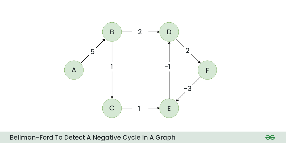
If such a cycle exists and is reachable from the source, there is no "shortest" path. You could traverse the cycle infinitely, making the path cost smaller and smaller, tending towards $-\infty$.

Bellman-Ford has a clever way to detect this. We've established that all simple shortest paths are found within $V-1$ iterations. So, what happens if we run the relaxation loop one more time—a $V$-th iteration?

• If no distances are updated during the $V$-th iteration, the graph is free of negative cycles, and the distances we found are correct.
• If any distance is updated during the $V$-th iteration, it means a shorter path has been found after the theoretical maximum for simple paths. This is only possible if the path involves a negative-weight cycle.

This simple check is the standard method for detecting negative cycles.

Implementation and Complexity Analysis

Let's consolidate the algorithm and look at its implementation and performance.

Algorithm Pseudocode:

1. Initialize dist array: dist[source] = 0, others ∞.
2. Relaxation Loop:
   for i from 1 to V-1:
for each edge (u, v) with weight w:
if dist[u] + w < dist[v]:
dist[v] = dist[u] + w
3. Negative Cycle Check:
   for each edge (u, v) with weight w:
if dist[u] + w < dist[v]:
// Negative cycle detected.
return "Graph contains a negative cycle"
4. Return dist array.

For a practical implementation, the cp-algorithms site provides a robust C++ example, including code to not just detect, but also reconstruct the negative cycle itself. This is an excellent resource for deeper study.

Given your full-stack background with JavaScript, you might also find this implementation from GeeksforGeeks helpful to see the logic in a familiar language.

Complexity Analysis

• Time Complexity: $O(V\cdot E)$
  The algorithm has two main parts: the relaxation loop and the cycle detection loop. The outer loop runs $V-1$ times (a factor of $V$), and the inner loop iterates through all $E$ edges. This gives $O(V\cdot E)$. The final check for negative cycles also iterates through all $E$ edges, which is $O(E)$. The dominant term is thus $O(V\cdot E)$.
• Space Complexity: $O(V+E)$
  We need $O(V)$ space for the distance array and $O(V+E)$ to store the graph itself (e.g., as a list of edges).

Compared to Dijkstra's $O(E\log V)$, Bellman-Ford is significantly slower, especially on dense graphs. This is the trade-off for its ability to handle negative weights.

Conclusion

Today you've added another fundamental graph algorithm to your toolkit. The Bellman-Ford algorithm addresses a critical gap left by Dijkstra's, equipping you to handle a wider range of graph problems.

Key Takeaways:

• Bellman-Ford solves the single-source shortest path problem for graphs that may include negative edge weights.
• Its core mechanic is to relax all edges in the graph for $V-1$ iterations.
• It can detect negative-weight cycles by running one additional iteration ($V$-th) and checking if any path can still be shortened.
• Its time complexity is $O(V\cdot E)$, making it slower than Dijkstra's. The choice between them is a classic architectural trade-off based on graph properties.

Preview of the Next Lesson:
We will shift our focus from finding paths to a different kind of graph optimization problem: finding a Minimum Spanning Tree (MST). An MST is a sub-graph that connects all vertices together with the minimum possible total edge weight, without forming any cycles. We will start by implementing Kruskal's algorithm, which uses a greedy approach and a special data structure called Union-Find to solve this problem efficiently.