Kruskal's Algorithm with Union-Find

The Greedy Strategy of Kruskal's Algorithm

Kruskal's algorithm works by building the MST piece by piece, always choosing the "cheapest" option available. The high-level strategy is as follows:

1. Create a list of all edges in the graph and sort them in non-decreasing order of their weight.
2. Iterate through the sorted edges.
3. For each edge, if adding it to our growing tree does not form a cycle, we add it. Otherwise, we discard it.
4. We stop once we have added $V-1$ edges, where $V$ is the number of vertices. At this point, all vertices will be connected.

This greedy choice of picking the smallest available edge at each step is guaranteed to produce a minimum spanning tree.

To see this process in action, the following video provides a clear visual introduction and a step-by-step walkthrough.

This brings up a critical question: how do we efficiently detect if adding an edge creates a cycle? This is where a specialized data structure becomes essential.

Cycle Detection with the Union-Find Data Structure

Checking for cycles every time we add an edge could be very slow if done naively (e.g., with a DFS or BFS). A much more efficient solution is to use the Union-Find data structure, also known as a Disjoint Set Union (DSU).

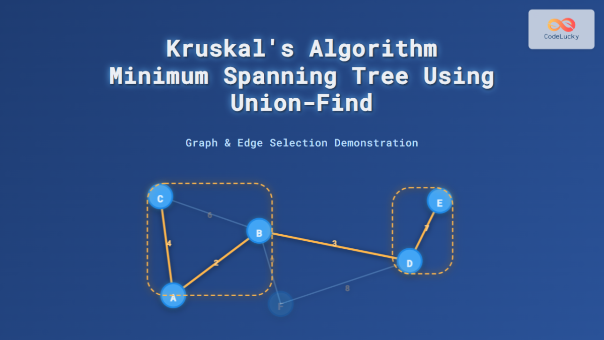
The core idea is to group vertices into sets, where each set represents a connected component of the forest we are building.

• Initially, each vertex is in its own set.
• When we consider adding an edge (u, v), we check which sets u and v belong to.
• If u and v are already in the same set, it means there's already a path between them. Adding the edge (u, v) would create a cycle. So, we discard the edge.
• If u and v are in different sets, adding the edge (u, v) will not create a cycle. It will simply connect two previously disconnected components. So, we add the edge to our MST and merge the two sets into one.

This structure primarily needs two operations:

1. find(i): Returns an identifier (or "root") for the set containing vertex i.
2. union(i, j): Merges the sets containing vertices i and j.

This next segment of the ByteQuest video explains how disjoint sets are used for cycle detection and introduces the underlying data structures (parent and rank arrays).

Optimizing Union-Find

A simple implementation of Union-Find can result in tall, "stringy" trees, making the find operation slow (potentially $O(V)$ in the worst case). Two powerful optimizations, Union by Rank and Path Compression, are used to flatten these trees and make operations nearly constant time on average.

• Union by Rank (or Size): When merging two sets, we attach the root of the smaller tree to the root of the larger tree. This keeps the overall tree depth low.
• Path Compression: During a find(i) operation, after finding the root, we make every node along the path from i to the root point directly to the root. This dramatically flattens the tree for future find calls involving those nodes.

The following video segments provide excellent visual explanations of these crucial optimizations.

Implementing Kruskal's Algorithm

Now we can combine the greedy strategy with our optimized Union-Find structure to build a complete implementation. Since you have a background as a software engineer, looking at a well-structured, class-based implementation can be very instructive.

The following article provides a clean Java implementation that encapsulates the logic in Edge, UnionFind, and KruskalAlgorithm classes. This approach is highly modular and reflects good software design principles.

The core logic within the main findMST method beautifully demonstrates the algorithm:

1. Sort all edges: Collections.sort(edges);
2. Initialize Union-Find: UnionFind uf = new UnionFind(vertices);
3. Iterate and build:

   for (Edge edge : edges) {
       int root1 = uf.find(edge.src);
       int root2 = uf.find(edge.dest);
       if (root1 != root2) { // Check if they are in different sets
           result.add(edge);  // Add edge to MST
           uf.union(root1, root2); // Merge the sets
       }
   }
   

Complexity Analysis

Understanding the performance characteristics of an algorithm is key to making informed architectural choices. Let's break down the complexity of Kruskal's algorithm, where $V$ is the number of vertices and $E$ is the number of edges.

• Time Complexity: $O(E\log E)$

  • Edge Sorting: The most computationally expensive step is sorting the list of $E$ edges. This takes $O(E\log E)$ time using an efficient sorting algorithm like Merge Sort or Quick Sort.
  • Union-Find Operations: We then iterate through each of the $E$ edges. For each edge, we perform up to two find operations and one union operation. With the path compression and union by rank optimizations, the amortized time for each operation is nearly constant, denoted as $O(\alpha (V))$, where $\alpha (V)$ is the extremely slow-growing inverse Ackermann function. For all practical purposes, you can think of this as $O(1)$.
  • Therefore, the total time for this phase is roughly $O(E\cdot \alpha (V))$.
  • The overall complexity is the sum of these parts: $O(E\log E+E\cdot \alpha (V))$. Since $\log E$ is much larger than $\alpha (V)$, the sorting step dominates. Thus, the final time complexity is $O(E\log E)$.

• Space Complexity: $O(V+E)$

  • We need $O(E)$ space to store the list of edges.
  • The UnionFind data structure requires $O(V)$ space for its parent and rank arrays.
  • Therefore, the total space complexity is $O(V+E)$.

The video from take U forward also has a good summary of the complexity analysis.

Conclusion

In this lesson, you've mastered Kruskal's algorithm, a fundamental tool for network optimization. This moves you beyond simple pathfinding into problems of structural connectivity.

Key Takeaways:

• Kruskal's algorithm finds a Minimum Spanning Tree by greedily adding the lowest-weight edges that do not form a cycle.
• The Union-Find (or Disjoint Set) data structure is the key to performing efficient cycle detection.
• Path Compression and Union by Rank are critical optimizations that make Union-Find operations nearly constant time on average.
• The algorithm's performance bottleneck is sorting the edges, leading to a time complexity of $O(E\log E)$.

Preview of the Next Lesson:
We will continue our exploration of Minimum Spanning Trees by implementing Prim's algorithm. While Kruskal's builds a "forest" of components that eventually merge, Prim's algorithm grows a single tree from a starting vertex, much like Dijkstra's algorithm. We will compare and contrast their approaches, performance, and ideal use cases.