Prim's Algorithm with Priority Queues

The Greedy Strategy of Prim's Algorithm

Prim's algorithm operates on a simple and intuitive greedy principle based on a graph theory concept called the "cut property."

In essence, Prim's algorithm works by maintaining a "cut" that separates the vertices already in the MST from those that are not. At each step, it finds the minimum-weight edge crossing this cut and adds it to the tree.

The high-level process is as follows:

1. Initialize an empty MST.
2. Choose an arbitrary starting vertex and add it to a set of "visited" vertices.
3. Add all edges connected to this starting vertex into a priority queue, which will store edges sorted by their weight.
4. While the MST doesn't yet include all vertices in the graph:
   a. Extract the edge with the minimum weight from the priority queue.
   b. If the vertex at the other end of this edge has not been visited yet, add the edge to our MST.
   c. Mark the newly added vertex as "visited" and add all of its outgoing edges that lead to unvisited vertices into the priority queue.
   d. If the destination vertex was already visited, we simply discard the edge and repeat step 4a. This prevents cycles.

Visualizing Prim's Algorithm

Watching the algorithm in action is the best way to solidify your understanding. The following video provides an excellent step-by-step walkthrough, showing how the priority queue and visited set evolve.

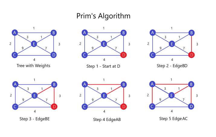
A key detail in the "lazy" version of Prim's algorithm (which is the most common implementation) is handling "stale" or "outdated" edges. A stale edge is one we pull from the priority queue that leads to a vertex we've already included in our MST via a different, cheaper path. Using a visited array allows us to efficiently detect and ignore these stale edges.

Implementing Prim's Algorithm

With a solid grasp of the logic, we can now turn to implementation. The core components are:

• An adjacency list to represent the graph.
• A min-priority queue to store potential edges, ordered by weight. In most languages, this will be a min-heap.
• A visited array (or set) to track vertices already in the MST.

The following resource provides clean, well-structured code in multiple languages. As a software engineer, you should be able to translate the logic across these examples.

The fundamental logic you'll see in the code follows this structure:

// Pseudocode for Prim's Algorithm
function prim(graph, startNode):
    pq = new PriorityQueue() // Stores {weight, destination_node}
    visited = new boolean[graph.numVertices]
    mst_total_weight = 0
    mst_edges = []

    // Start the algorithm
    pq.add({0, startNode}) // Add a dummy edge to kick things off

    while pq is not empty:
        {weight, u} = pq.extractMin()

        if visited[u]:
            continue // Ignore stale edge

        visited[u] = true
        mst_total_weight += weight
        // If you need the edge itself, you'd store the parent and add {parent, u} to mst_edges

        for each neighbor v of u with edge_weight w:
            if not visited[v]:
                pq.add({w, v})

    return mst_total_weight

Complexity Analysis

Understanding the performance of Prim's algorithm is crucial for deciding when to use it over Kruskal's. Let $V$ be the number of vertices and $E$ be the number of edges.

• Time Complexity: $O(E\log V)$ or $O(E\log E)$

  • The main while loop can run up to $E$ times in the worst case because we might add all edges to the priority queue.
  • Each operation on the priority queue (insertion and extraction) takes $O(\log N)$ time, where $N$ is the number of items in the queue. In our case, the queue size can grow up to $E$. So, the complexity of PQ operations is $O(\log E)$.
  • Since $E$ can be at most $V(V-1)/2\approx V^2$, we have $\log E\approx \log (V^2)=2\log V$. Therefore, $\log E$ is in $O(\log V)$.
  • Combining these, the total time complexity is dominated by the priority queue operations over all edges, giving us $O(E\log V)$.

• Space Complexity: $O(V+E)$

  • The adjacency list requires $O(V+E)$ space.
  • The visited array requires $O(V)$ space.
  • In the worst case (a dense graph), the priority queue might need to store an edge for every connection, leading to $O(E)$ space.
  • Therefore, the total space complexity is $O(V+E)$.

The following video provides a concise summary of this analysis.

Conclusion

You have now implemented the two most famous algorithms for finding a Minimum Spanning Tree. This gives you a powerful set of tools for solving network optimization problems where the goal is total connectivity with minimum cost.

Key Takeaways:

• Prim's algorithm finds an MST by greedily growing a single tree from a starting vertex.
• It relies on the cut property: always add the minimum-weight edge that connects a visited vertex to an unvisited one.
• An efficient implementation uses a priority queue to quickly find this minimum-weight edge and a visited array to prevent cycles and ignore stale edges.
• The time complexity is $O(E\log V)$, making it very efficient, especially for dense graphs where $E$ is close to $V^2$.

Preview of the Next Lesson:
You've now implemented four major graph algorithms: Dijkstra's, Bellman-Ford, Kruskal's, and Prim's. In our next lesson, we will step back from implementation and move towards architectural thinking. We will compare and contrast these algorithms, discussing their specific use cases, constraints (e.g., negative weights, graph density), and performance trade-offs. This will equip you to make informed decisions about which algorithm to apply to a given design problem.