Dijkstra's Algorithm: Finding the Shortest Path

The Single-Source Shortest Path Problem

Before diving into the algorithm, let's define the problem it solves: the Single-Source Shortest Path (SSSP) problem.

Given:

1. A weighted graph, where edges have a numerical value (cost, distance, time, etc.). For now, we'll assume these weights are non-negative.
2. A designated source vertex, s.

The goal is to find the shortest path from the source vertex s to every other vertex in the graph.

To get a formal understanding of the SSSP problem and the terminology we'll be using, the VisuAlgo resource is an excellent starting point.

The Core Idea: A Greedy Strategy

Dijkstra's algorithm works by progressively finding the shortest path to the "closest" vertices first. It's a greedy algorithm because at each step, it makes the locally optimal choice: it explores the unvisited vertex that has the smallest known distance from the source.

To do this, the algorithm maintains a few key pieces of information:

• A set of visited vertices whose shortest path from the source is considered final.
• A distance array/map, let's call it dist, where dist[v] stores the length of the shortest path currently known from the source to vertex v. Initially, dist[source] = 0 and all other distances are set to infinity.
• A priority queue containing unvisited vertices, prioritized by their current value in the dist array. This is the crucial data structure that allows us to efficiently select the "closest" unvisited vertex at each step.

The algorithm proceeds as follows:

1. Initialize dist for all vertices and add the source vertex to the priority queue with a distance of 0.
2. While the priority queue is not empty:
   a. Extract the vertex u with the minimum distance from the priority queue.
   b. Mark u as visited. Its shortest path is now considered final.
   c. For each neighbor v of u, perform a "relaxation" step.

The "Relaxation" Step

Relaxation is the heart of the algorithm. For an edge from u to v with weight w, we check if we've found a shorter path to v by going through u. The logic is simple:

If dist[u] + w < dist[v], it means the path from the source to v via u is shorter than any path to v we've found so far. So, we update dist[v] to this new, shorter distance: dist[v] = dist[u] + w.

Visualizing Dijkstra's Algorithm

Theory is one thing, but seeing the algorithm unfold is the best way to build intuition. The following video provides a clear, step-by-step visualization.

From Concept to Code

As a software engineer, you know the gap between a conceptual algorithm and a working implementation. Let's bridge that gap.

A key implementation detail concerns the priority queue. During the relaxation step, if we find a shorter path to a vertex v that's already in the priority queue, we need to update its priority (its distance). This operation is often called decrease-key. However, many standard library priority queue implementations (like Python's heapq or Java's PriorityQueue) don't offer a direct and efficient decrease-key method.

The common and practical solution is a "lazy update" approach:

• Instead of trying to update an existing entry in the priority queue, we simply add a new (new_distance, vertex) pair.
• This means the queue might temporarily contain multiple entries for the same vertex with different distances.
• When we extract an item (distance, vertex) from the queue, we first check if we have already found a shorter path to that vertex. If the extracted distance is greater than the value we have stored in our dist array for that vertex, it's an outdated entry, and we simply ignore it and extract the next item.

This video from NeetCode demonstrates this practical implementation style.

For your reference, here is a resource with full code examples in multiple languages. You can review the language of your choice to solidify your understanding.

Test your understanding!

Consider the graph below, with A as the source vertex.

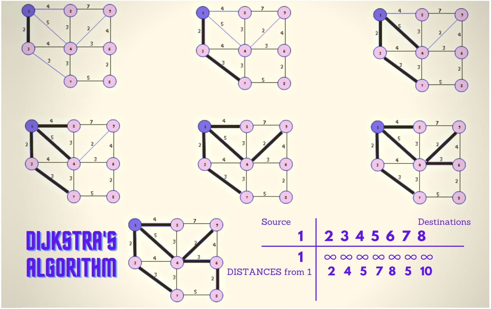
Trace the first few steps of Dijkstra's algorithm.

1. What is the state of the dist array and the priority queue after initialization?
2. Which node is extracted first? What updates are made?
3. Which node is extracted second? What updates are made?

Show answer

Let's use the node numbers from the image (1=A, 2=B, etc.), with Node 1 as the source.

1. Initialization:

   • dist array: [0, ∞, ∞, ∞, ∞, ∞, ∞, ∞]
   • Priority Queue pq: [(0, 1)]

2. First Extraction:

   • Extract (0, 1) from pq.
   • Neighbors of 1 are 2 and 3.
   • Relax edge (1, 2) with weight 2: dist[1] + 2 < dist[2] (0+2 < ∞). Update dist[2] = 2. Push (2, 2) to pq.
   • Relax edge (1, 3) with weight 4: dist[1] + 4 < dist[3] (0+4 < ∞). Update dist[3] = 4. Push (4, 3) to pq.
   • dist array is now: [0, 2, 4, ∞, ∞, ∞, ∞, ∞]
   • pq is now: [(2, 2), (4, 3)]

3. Second Extraction:

   • Extract (2, 2) from pq (since 2 is the minimum distance).
   • Neighbors of 2 are 3, 4, and 5.
   • Relax edge (2, 3) with weight 3: dist[2] + 3 < dist[3] (2+3 < 4) is FALSE. No update for node 3.
   • Relax edge (2, 4) with weight 7: dist[2] + 7 < dist[4] (2+7 < ∞). Update dist[4] = 9. Push (9, 4) to pq.
   • Relax edge (2, 5) with weight 5: dist[2] + 5 < dist[5] (2+5 < ∞). Update dist[5] = 7. Push (7, 5) to pq.
   • dist array is now: [0, 2, 4, 9, 7, ∞, ∞, ∞]
   • pq is now: [(4, 3), (9, 4), (7, 5)] (ordered by distance)

Complexity and a Critical Limitation

As requested, let's analyze the complexity. The efficiency of Dijkstra's hinges on the priority queue.

• Time Complexity: $O((V+E)\log V)$

  • We extract each of the $V$ vertices from the priority queue once. Each extraction (extract-min) costs $O(\log V)$. Total: $O(V\log V)$.
  • In the worst case, we might relax every edge. Each relaxation could lead to an insertion into the priority queue (push or decrease-key), which costs $O(\log V)$. Total for all edges: $O(E\log V)$.
  • Combining these gives a total time complexity of $O(V\log V+E\log V)$, which is often written as $O((V+E)\log V)$. For connected graphs, $E$ is at least $V-1$, so this is commonly simplified to $O(E\log V)$.

• Space Complexity: $O(V+E)$

  • We need space for the dist and predecessor arrays, which is $O(V)$.
  • The adjacency list representation of the graph takes $O(V+E)$ space.
  • The priority queue can, in the worst case (with the lazy update method), hold an entry for each edge, taking $O(E)$ space.

Limitation: Negative Edge Weights
Dijkstra's greedy approach relies on a critical assumption: all edge weights are non-negative. This guarantees that once a vertex is extracted from the priority queue and marked as visited, we have found its true shortest path.

If a graph has a negative edge, this assumption breaks. A path that currently looks longer might eventually lead to a negative edge, making it shorter in the end. Dijkstra's algorithm, having already finalized a "shorter" path greedily, would miss this.

Conclusion

You have now learned one of the most important graph algorithms in computer science. Dijkstra's algorithm provides an efficient way to solve the single-source shortest path problem, a task that underlies many modern technologies.

Key Takeaways:

• Dijkstra's algorithm finds the shortest path from a source to all other nodes in a non-negatively weighted graph.
• It uses a greedy strategy, always exploring the unvisited node with the smallest known distance.
• A priority queue is essential for an efficient implementation, with a time complexity of $O((V+E)\log V)$.
• The "lazy update" method is a common way to implement Dijkstra's without needing a complex decrease-key operation in the priority queue.
• The algorithm's greedy nature is its weakness: it fails on graphs with negative edge weights.

Preview of the Next Lesson:
The limitation we just discussed sets the stage perfectly for our next topic. We will explore the Bellman-Ford algorithm. While slower than Dijkstra's, it is more robust as it can handle graphs with negative edge weights and has the added ability to detect negative-weight cycles, a scenario where the "shortest path" is undefined.