Unitarity and Operator Dimensions

1. Unitarity, Reflection Positivity, and Radial Quantization

In a Lorentzian quantum field theory, unitarity implies that the Hamiltonian is Hermitian and that the Hilbert space has a positive-definite norm. Since we are working in Euclidean signature, this principle takes a slightly different, but equivalent, form known as reflection positivity.

In the context of radial quantization, where we think of states as being created by operators at the origin, the Hilbert space is the set of states $|\mathcal{O}\rangle = \mathcal{O}(0)|0\rangle$. The inner product $\langle \psi | \phi \rangle$ must be well-defined and the norm $\langle \psi | \psi \rangle$ must be non-negative.

This requirement leads to a specific definition of the Hermitian conjugate $\dagger$ for operators and generators in radial quantization. The conjugate of an operator $\mathcal{O}(x)$ turns out to be related to its transformation under inversion $I$:

For the generators of the conformal algebra, this implies the following crucial relations:

• $D^\dagger = D$ (Dilatation operator is Hermitian)
• $M_{\mu\nu}^\dagger = -M_{\mu\nu}$ (Rotation generators are anti-Hermitian, as expected)
• $P_\mu^\dagger = K_\mu$ (The translation generator is the adjoint of the special conformal generator!)

This last relation, $P_\mu^\dagger = K_\mu$, is the key to deriving the unitarity bounds.

2. Deriving the Unitarity Bounds

With the conjugation rules established, we can now derive constraints on $\Delta$ by demanding that all states in the Hilbert space have non-negative norms. We start with a primary state $|\mathcal{O}\rangle$, defined by $K_\mu |\mathcal{O}\rangle = 0$ and $D|\mathcal{O}\rangle = \Delta |\mathcal{O}\rangle$ and then compute the norm of its descendants.

The Scalar Case ($\ell=0$)

Let $|\mathcal{O}\rangle$ be a scalar primary state. Let's compute the norm-squared of its simplest descendant, $| \psi \rangle = P_\nu |\mathcal{O}\rangle$:

Since $|\mathcal{O}\rangle$ is a primary state, `$K_{\nu }$ annihilates it. We can therefore insert the commutator:

Using the conformal algebra commutator $[K_\mu, P_\nu] = 2\delta_{\mu\nu}D - 2M_{\mu\nu}$ (in Euclidean signature, with $M$ anti-hermitian), we get:

(The $M_{\nu\nu}$ term is zero). Since we must have $\langle \psi | \psi \rangle \ge 0$ and we can normalize $\langle \mathcal{O} | \mathcal{O}\rangle > 0$, this implies:

The case $\Delta=0$ corresponds to the identity operator, which is translationally invariant ($P_\nu|I\rangle = 0$), so its descendants have zero norm trivially.

By considering more complex descendants, we can derive stronger bounds.

As the text explains, a more detailed analysis yields the complete set of unitarity bounds for primary operators represented by symmetric traceless tensors in $d$ dimensions:

• Scalar operators ($\ell=0$):
  • $\Delta = 0$ (This is the identity operator $I$).
  • $\Delta \ge \frac{d-2}{2}$ (All other scalar primaries).
• Spinning operators ($\ell>0$):
  • $\Delta \ge \ell + d - 2$

Any operator in a unitary CFT must have a $(\Delta, \ell)$ pair that satisfies these inequalities. This is a profound constraint on the spectrum of possible theories.

3. Null States and Saturating the Bounds

What happens when an operator's dimension lies exactly on the boundary of the allowed region? In this case, the norm of some descendant state becomes zero. A state with zero norm is called a null state or null vector.

In a unitary theory, null states are physically unobservable and must be set to zero. This condition $|\text{null state}\rangle = 0$ translates into a differential equation for the corresponding operator $\mathcal{O}(x)$.

• Free Scalar: For a scalar $\mathcal{O}$ saturating the bound $\Delta = \frac{d-2}{2}$, the null state is $P^2|\mathcal{O}\rangle$ at level 2. The condition $P^2|\mathcal{O}\rangle = 0$ corresponds to the operator equation $\partial^2 \mathcal{O}(x) = 0$. This is the equation of motion for a free, massless scalar field.

• Conserved Currents: For a spin-$\ell$ operator $\mathcal{O}_{\mu_1 \dots \mu_\ell}$ saturating the bound $\Delta = \ell + d - 2$, a null state appears at level 1. This leads to the operator equation $\partial^{\mu_1} \mathcal{O}_{\mu_1 \dots \mu_\ell}(x) = 0$. This is the condition for a conserved current.

  • For $\ell=1$, we get a conserved vector current $J_\mu$ with $\Delta = d-1$.
  • For $\ell=2$, we get the conserved stress-energy tensor $T_{\mu\nu}$ with $\Delta = d$. This is a universal operator present in any CFT.

Conclusion

In this lesson, we have seen how the fundamental requirement of unitarity, via reflection positivity in radial quantization, leads to powerful, universal constraints on the spectrum of any CFT.

Key Takeaways:

• Unitarity and Norms: Unitarity implies that all states in the Hilbert space must have non-negative norms.
• $P^\dagger=K$ is Key: The conjugation property $P_\mu^\dagger = K_\mu$ allows us to calculate the norms of descendant states in terms of the primary state's dimension $\Delta$.
• Unitarity Bounds: Demanding non-negative norms for all descendants forces the dimensions of primary operators to obey strict lower bounds that depend on their spin $\ell$ and the spacetime dimension $d$.
  • $\Delta \ge (d-2)/2$ for scalars ($\ell=0$).
  • $\Delta \ge \ell + d - 2$ for spin $\ell > 0$.
• Null States and Conservation: Operators that saturate these bounds contain null states in their Verma module. In a unitary theory, these null states must vanish, which imposes differential equations on the operators, turning them into conserved currents or free fields.

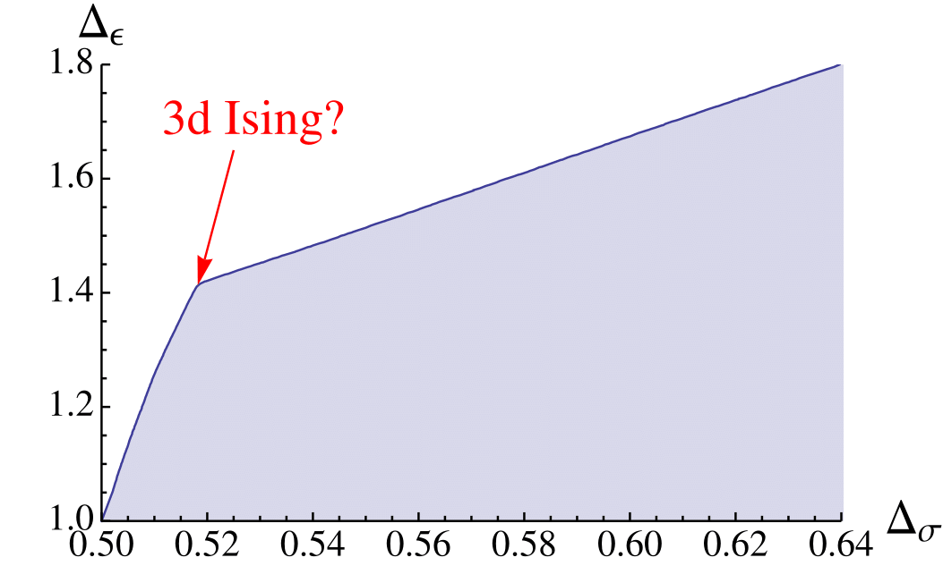
These bounds are not just theoretical niceties; they are the bedrock of the numerical bootstrap. They define the allowed "search space" for the operator dimensions $\Delta$ that can appear in the bootstrap equation, making the problem of finding a separating functional a well-posed and tractable task.

Next Lesson Preview:
We now have all the conceptual pieces of the modern bootstrap in place: the bootstrap equation from crossing symmetry, and the unitarity bounds that constrain the spectrum. In the next lesson, we will begin our dive into the numerical implementation. We will see how to formulate the bootstrap as a concrete numerical optimization problem, seeking the "separating functional" that we discussed, and how this leads to powerful, rigorous bounds on CFT data.