Hello! Welcome back to our exploration of the modern conformal bootstrap.
In our last lesson, we established a crucial result: the four-point function, which conformal symmetry alone leaves partially undetermined, can be decomposed into a sum over universal kinematic objects called conformal blocks. This conformal partial wave expansion, $g(u, v) = \sum_{\mathcal{O}} f_{\phi\phi\mathcal{O}}^2 g_{\Delta_{\mathcal{O}}, \ell_{\mathcal{O}}}(u, v)$, separates the theory-dependent data ($\Delta, \ell, f$) from the universal structure of the theory.
Today, we will introduce the final two ingredients—crossing symmetry and unitarity—to assemble the fundamental bootstrap equations. Your goal for this lesson is to learn how to apply these constraints to derive the equations that form the bedrock of the entire bootstrap program. This will shift our perspective from merely describing CFT correlators to actively constraining the space of all possible CFTs.
1. OPE Associativity and Crossing Symmetry
The conformal block expansion we derived was based on a choice: we grouped operators $\phi(x_1)$ with $\phi(x_2)$ and $\phi(x_3)$ with $\phi(x_4)$ before applying the Operator Product Expansion (OPE). This is often called the "s-channel" decomposition.
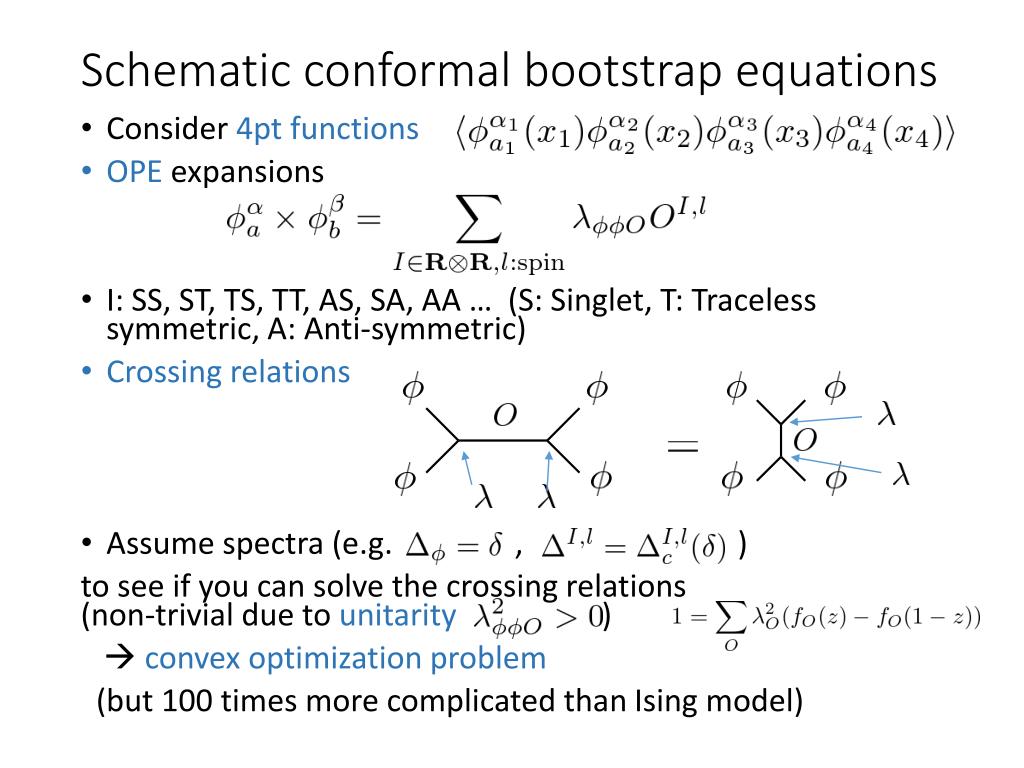
However, the correlation function $\langle \phi(x_1)\phi(x_2)\phi(x_3)\phi(x_4) \rangle$ is a single, unambiguous physical quantity. Its value cannot depend on the order in which we choose to fuse operators. We could just as well have grouped $\phi(x_1)$ with $\phi(x_4)$ and $\phi(x_2)$ with $\phi(x_3)$ (the "t-channel"), or $\phi(x_1)$ with $\phi(x_3)$ and $\phi(x_2)$ with $\phi(x_4)$ (the "u-channel"). This is a statement about the associativity of the OPE: $(\phi_1 \phi_2) \phi_3 = \phi_1 (\phi_2 \phi_3)$.
Requiring that these different ways of computing the correlator give the same result leads to a powerful self-consistency condition known as crossing symmetry.
TASI Lectures on the Conformal Bootstrap
Let's begin with David Simmons-Duffin's 'TASI Lectures on the Conformal Bootstrap' to see how OPE associativity is formally expressed as the crossing symmetry equation.
Please read Section 10.1, 'OPE Associativity and Crossing Symmetry' (pages 49-51). Focus on the logic leading to equation (182), which equates the block expansion in two different channels. The diagrams in this section provide a very clear intuition for this equivalence.
As the notes show, equating the s-channel expansion (12) \to (34) with the t-channel expansion (14) \to (23) gives the crossing equation. For a four-point function of identical scalars $\phi$, this takes the form of a simple-looking identity for the function $g(u,v)$:
This equation might seem unassuming, but when we substitute the conformal block expansion into it, it becomes a profound constraint on the CFT data.
2. The Fundamental Bootstrap Equation
Let's now write out the crossing equation explicitly using the conformal block expansion. We have two expressions for the four-point function:
- s-channel expansion (pairing 1-2, 3-4):
- t-channel expansion (pairing 2-3, 1-4):
Equating these two and rearranging using the definitions of $u$ and $v$ gives our constraint on $g(u,v)$. Combining this with the block expansion yields:
This can be rewritten in a more suggestive form:
This is the fundamental bootstrap equation. It is a sum over the entire spectrum of the theory, and it must hold for all $u, v$. Before we analyze its power, we must incorporate the second key ingredient: unitarity.
TASI Lectures on the Conformal Bootstrap
The bootstrap equation is subject to several constraints, most of which stem from unitarity. The Simmons-Duffin notes conveniently summarize these for our case of identical scalars.
Please read Section 10.2, 'Crossing Symmetry for Identical Scalars' (pages 52-53). This section lists the crucial properties that any unitary CFT must obey, such as the reality and positivity of $f_{\phi\phi\mathcal{O}}^2$ and the unitarity bounds on operator dimensions. Pay close attention to equation (186) and the properties listed below it.
As a reminder, the essential unitarity constraints are:
- Positivity of OPE coefficients: In a unitary theory, we can choose a basis where the OPE coefficients
$f_{\phi\phi\mathcal{O}}$are real. Therefore, their squares$f_{\phi\phi\mathcal{O}}^2$are non-negative. We will denote$p_{\mathcal{O}} = f_{\phi\phi\mathcal{O}}^2 \ge 0$. - Unitarity Bounds: The dimension
$\Delta$and spin$\ell$of any primary operator$\mathcal{O}$(except the identity) must satisfy$\Delta \ge \ell + d - 2$for$\ell > 0$and$\Delta \ge \frac{d-2}{2}$for$\ell = 0$. - Spectrum: The OPE of two identical scalars
$\phi \times \phi$can only contain operators$\mathcal{O}$with even spin$\ell$.
3. The Logic of Constraining CFT Data
The bootstrap equation, combined with the unitarity constraints, provides a powerful tool for constraining CFT data. Let's rewrite the equation abstractly.
Let $\vec{F}_{\Delta, \ell}$ be a vector in the infinite-dimensional space of functions of $(u, v)$:
The bootstrap equation is then a simple statement about a sum of these vectors:
The sum runs over all primary operators $(\Delta, \ell)$ in the $\phi \times \phi$ OPE. This includes the identity operator, $(\Delta=0, \ell=0)$, for which $p_{0,0} = f_{\phi\phi I}^2 = 1$. The equation states that the "bootstrap vectors" $\vec{F}_{\Delta, \ell}$ must sum to zero with positive coefficients. This is a very strong constraint.
This geometric picture allows us to rule out hypothetical CFTs.
TASI Lectures on the Conformal Bootstrap
The insight of the modern bootstrap was to turn this problem around: instead of trying to solve the equation for a specific theory, one asks which hypothetical sets of CFT data cannot satisfy the equation. This leads to rigorous bounds on the properties of all CFTs.
Please read Section 10.4, 'Bounds on CFT Data' (page 54), focusing on Algorithm 1 and the logic illustrated in Figure 25. Understand how the existence of a 'separating plane' (a linear functional $\alpha$ ) can lead to a contradiction, thereby ruling out a hypothesized operator spectrum.
The logic is as follows:
- Make a hypothesis about the CFT spectrum. For example: "Assume there is no scalar operator with dimension
$\Delta < \Delta^*$in the$\phi \times \phi$OPE, other than the identity." - Search for a separating functional. This is a linear functional
$\alpha$(a linear map from the space of functions to the real numbers) that acts on our bootstrap vectors. We search for an$\alpha$with two properties:$\alpha(\vec{F}_{\text{identity}}) > 0$$\alpha(\vec{F}_{\Delta, \ell}) \ge 0$for all operators$(\Delta, \ell)$allowed by our hypothesis.
- Look for a contradiction. If such an
$\alpha$exists, we can apply it to the bootstrap equation: But wait! The sum is$p_{0,0} \alpha(\vec{F}_{0,0}) + \sum_{\text{others}} p_{\Delta, \ell} \alpha(\vec{F}_{\Delta, \ell})$. We have$p_{0,0}=1$and we chose$\alpha(\vec{F}_{0,0}) > 0$. All other$p_{\Delta, \ell}$are$\ge 0$and we required$\alpha(\vec{F}_{\Delta, \ell}) \ge 0$. The sum must therefore be strictly positive! This is a contradiction ($0 > 0$). Therefore, our initial hypothesis must be false. We have rigorously proven that a CFT with the assumed properties cannot exist.
This method allows us to carve out the space of allowed CFT data by ruling out everything else.
Test your understanding!
Consider a simplified problem in a 2D vector space. Let the bootstrap vectors be $\vec{v}_1 = (1, 1)$, $\vec{v}_2 = (1, -2)$, and $\vec{v}_3 = (-3, 0)$. Can these three vectors satisfy a bootstrap-like equation $p_1 \vec{v}_1 + p_2 \vec{v}_2 + p_3 \vec{v}_3 = \vec{0}$ with $p_1, p_2, p_3 > 0$? (This is asking if the origin is in the convex hull of the vectors).
Show answer
Yes, they can. For example, $p_1 = 6$, $p_2 = 3$, $p_3 = 3$ is a solution:$6(1, 1) + 3(1, -2) + 3(-3, 0) = (6, 6) + (3, -6) + (-9, 0) = (9, 0) + (-9, 0) = (0, 0)$.
Now, consider a different set of vectors: $\vec{w}_1 = (1, 1)$, $\vec{w}_2 = (2, 1)$, and $\vec{w}_3 = (1, -1)$. Can these sum to zero with positive coefficients?
No. All these vectors lie in the half-plane $x > 0$ (except $\vec{w}_3$ which lies on the boundary $x > 0$ if we only consider its x-component). A linear combination with positive coefficients will always have a positive x-component. The functional $\alpha(\vec{w}) = w_x$ is a separating functional: $\alpha(\vec{w}_i) > 0$ for all $i$. Thus $\sum p_i \alpha(\vec{w}_i) > 0$, leading to a contradiction.
Conclusion
This lesson has been pivotal. We have assembled the core machinery of the conformal bootstrap. By demanding that the OPE be associative (crossing symmetry) and that the theory be unitary, we derived the fundamental bootstrap equation.
Key Takeaways:
- Crossing Symmetry: The requirement that the four-point function is independent of the OPE channel (
svst) provides a powerful functional equation. - The Bootstrap Equation: The crossing symmetry equation, written in terms of conformal blocks, is
$\sum p_{\Delta, \ell} \vec{F}_{\Delta, \ell} = 0$, where$\vec{F}_{\Delta, \ell}$are known kinematic functions and$p_{\Delta, \ell} = f_{\phi\phi\mathcal{O}}^2 \ge 0$are the squared OPE coefficients. - The Bootstrap Logic: This equation states that a set of known vectors must sum to zero with positive coefficients. This geometric constraint is incredibly powerful and allows us to derive rigorous bounds on CFT data (
$\Delta, \ell, f$) by finding separating functionals that rule out hypothesized spectra.
Next Lesson Preview:
We have established the logic of the bootstrap. In the next lesson, we will begin to explore its consequences. We will delve into the properties of the bootstrap vectors $\vec{F}_{\Delta, \ell}$ and see how the unitarity bounds on $\Delta$ and $\ell$ constrain their behavior, making the search for separating functionals a well-posed problem. This will set the stage for understanding how the first numerical bootstrap bounds were obtained.