Conformal Bootstrap: Numerical Optimization for CFT Data

1. From an Equation to a Geometric Constraint

Let's begin by re-interpreting the bootstrap equation. It states that a set of vectors $\vec{F}_{\Delta, \ell}$, corresponding to the primary operators in the theory, must sum to zero with positive coefficients $p_{\mathcal{O}} = \lambda_{\phi\phi\mathcal{O}}^2 \ge 0$. Geometrically, this means that the origin of our vector space must lie within the convex cone spanned by the vectors $\{\vec{F}_{\Delta, \ell}\}$.

This geometric picture provides a powerful way to test if a hypothetical set of operators could exist in a CFT.

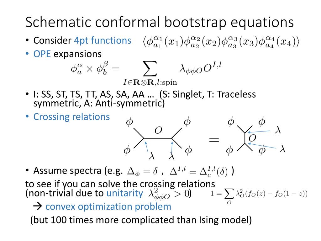
Imagine you hypothesize a certain spectrum of operators—for example, "in the OPE of a scalar $\phi$ with itself, all other scalar operators $\mathcal{O}$ have dimension $\Delta_{\mathcal{O}} \ge 5$". Can such a theory exist?

The bootstrap provides a definitive test: if we can find a "separating plane" (a hyperplane through the origin) such that all vectors $\vec{F}_{\Delta, \ell}$ corresponding to our hypothesized spectrum lie on one side of it, then it's impossible for any positive linear combination of them to sum to zero. The existence of such a plane proves the hypothesis is false.

This "separating plane" is mathematically represented by a linear functional, which we can call $\alpha$. A linear functional is an object that takes a vector and returns a number, $\alpha(\vec{F})$. The condition that all vectors lie on one side of the plane translates to $\alpha(\vec{F}_{\Delta, \ell}) \ge 0$.

As the text explains, this gives us a clear algorithm:

1. Make a hypothesis about the spectrum of operators appearing in the OPE (e.g., a lower bound on the dimension of the first scalar operator).
2. Search for a linear functional $\alpha$ such that:
   • $\alpha(\vec{F}_{\Delta, \ell}) \ge 0$ for all $(\Delta, \ell)$ allowed by the hypothesis and unitarity.
   • $\alpha(\vec{F}_{id}) > 0$ for the identity operator's contribution (or another operator guaranteed to be present).
3. If such an $\alpha$ exists, the hypothesis is impossible. Applying $\alpha$ to the bootstrap equation $\sum p_{\mathcal{O}} \vec{F}_{\mathcal{O}} = 0$ leads to a contradiction: a sum of non-negative numbers (with at least one strictly positive term) cannot be zero.

2. Making the Problem Finite and Computable

This algorithm is elegant, but it faces two immediate computational challenges:

1. The space of possible functionals $\alpha$ is infinite-dimensional.
2. The number of positivity constraints $\alpha(\vec{F}_{\Delta, \ell}) \ge 0$ is infinite, since the spin $\ell$ can be arbitrarily large and the dimension $\Delta$ is a continuous variable.

To make this tractable for a computer, we must make the problem finite.

Dealing with the functional $\alpha$:
We restrict our search for $\alpha$ to a finite-dimensional subspace. A standard and effective choice is to define $\alpha$ by a finite number of derivatives of the crossing equation around the "crossing-symmetric point" ($z = \bar{z} = 1/2$). The functional is then parameterized by a finite set of coefficients $a_{mn}$:

Our search for an abstract functional $\alpha$ is now a search for the numbers $a_{mn}$. The larger the cutoff $\Lambda$, the more powerful our search, but the more computationally intensive it becomes.

Dealing with the constraints:
The infinite number of constraints is more subtle. We have $\alpha(\vec{F}_{\Delta, \ell}) \ge 0$ for every $\ell \in \{0, 2, 4, ...\}$ and for a continuous range of $\Delta$ above the unitarity bound for that spin.

• For spin $\ell$, one can often handle the infinite sum by imposing constraints up to some $\ell_{\max}$ and then proving that the positivity holds for $\ell > \ell_{\max}$ analytically.
• For the continuous variable $\Delta$, we cannot simply discretize it and check a finite number of points, as we might miss a point where the function dips below zero. We need a way to enforce positivity over a continuous interval.

This is where the structure of conformal blocks and a powerful optimization technique come into play.

3. Semidefinite Programming: The Engine of the Bootstrap

As the notes mention, the key is to formulate our problem in a language that computers can solve efficiently. The problem of finding coefficients $a_{mn}$ such that a function remains positive over an interval is perfectly suited for semidefinite programming (SDP).

The core idea is as follows:

1. The quantities we are constraining, $\partial_z^m \partial_{\bar{z}}^n F_{\Delta, \ell}$, are complicated functions of $\Delta$. However, they can be written or well-approximated as polynomials in $\Delta$ divided by a positive function.
2. Our constraint $\alpha(F_{\Delta, \ell}) \ge 0$ thus becomes a condition that a certain polynomial in $\Delta$ (whose coefficients depend linearly on our unknown $a_{mn}$'s) must be non-negative for all $\Delta$ above the unitarity bound.
3. A famous result in mathematics states that a polynomial which is non-negative on a given domain can be written as a sum of squares of other polynomials.
4. The condition that a polynomial can be written as a sum of squares can be translated into the condition that a certain matrix (built from the polynomial's coefficients) is positive semidefinite.

This transforms our problem into the canonical form of an SDP: "Find a vector $\vec{a}$ (our $a_{mn}$ coefficients) such that a set of matrices $M_i(\vec{a})$ are all positive semidefinite." This is a convex optimization problem, for which efficient and reliable algorithms exist.

Conclusion

We have now seen how the abstract principles of conformal symmetry and unitarity are forged into a powerful computational tool. By turning a physics problem into a question of geometry and then into a standard numerical optimization problem, we can derive rigorous, non-perturbative results about quantum field theories.

Key Takeaways:

• The bootstrap equation $\sum p_{\mathcal{O}} \vec{F}_{\mathcal{O}} = 0$ with $p_{\mathcal{O}} \ge 0$ means the origin must lie in the convex cone of the vectors $\vec{F}_{\mathcal{O}}$.
• We can rule out a hypothetical spectrum by finding a separating functional $\alpha$ that is positive on all vectors corresponding to that spectrum.
• The infinite-dimensional search for $\alpha$ is made finite by restricting it to a space of derivatives at the crossing-symmetric point.
• The problem of enforcing positivity constraints over a continuous range of operator dimensions $\Delta$ is solved by reformulating it as a semidefinite program (SDP), which can be solved efficiently on a computer.

Next Lesson Preview:
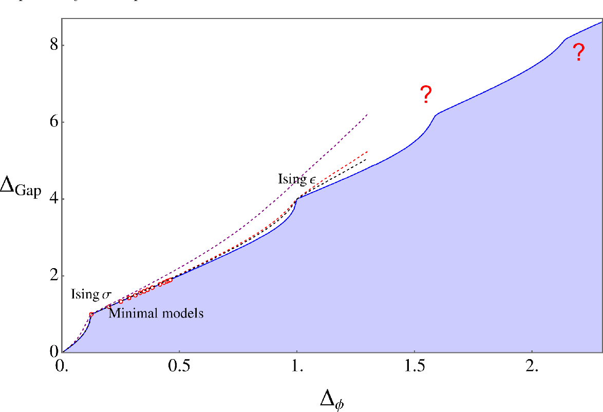
Now that we understand the machinery that produces bootstrap results, we will learn how to interpret its output. The results of a numerical bootstrap run are typically presented as exclusion plots. In the next lesson, we will examine these plots, understand what they represent, and see how features like "kinks" and "islands" can be used to pinpoint the precise location of specific CFTs, like the celebrated 3D Ising model.