Hello! Welcome to the culmination of our study of the modern conformal bootstrap.
In the previous lesson, we constructed the computational engine of the bootstrap. We saw how the abstract principles of crossing symmetry and unitarity can be transformed into a concrete numerical procedure—semidefinite programming (SDP). This procedure acts as an oracle: we propose a hypothesis about the spectrum of a CFT (e.g., "the lightest scalar operator \mathcal{O} has dimension \Delta_{\mathcal{O}} \ge \Delta_{\text{test}}"), and the SDP solver tells us whether this hypothesis is consistent with the axioms.
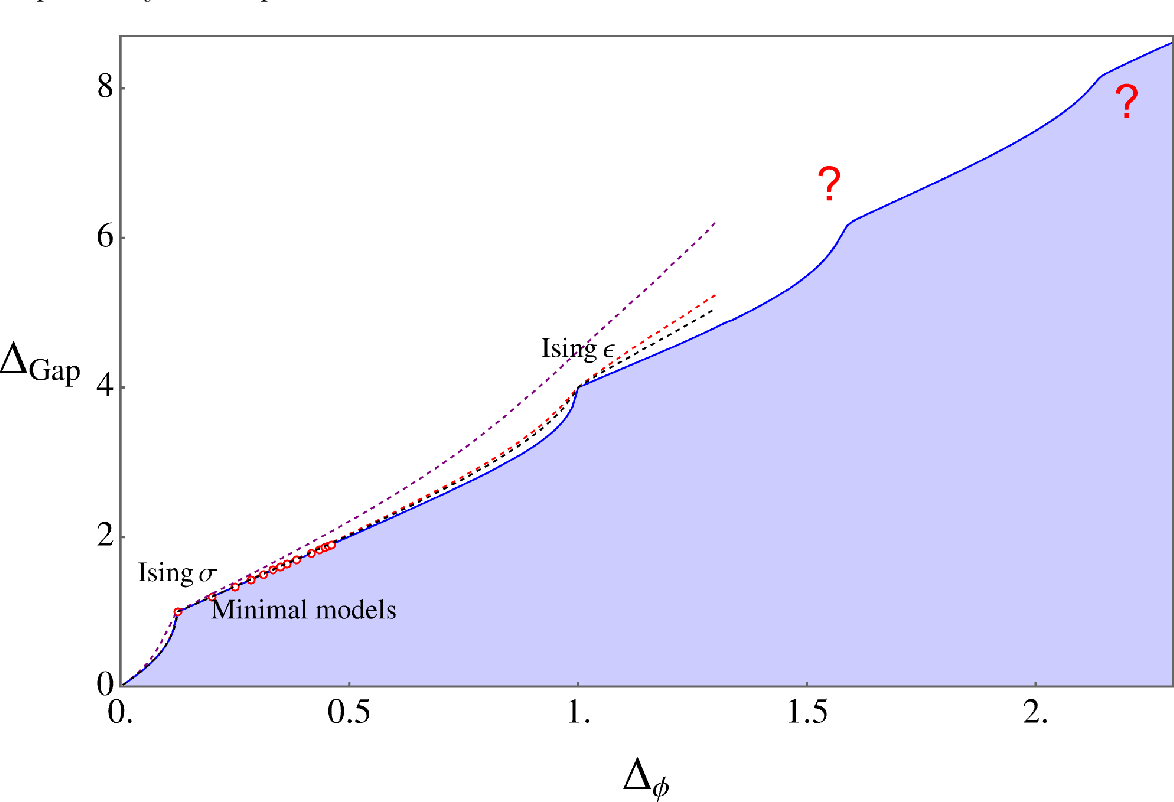
Today, we will learn how to use the output of this oracle to derive powerful, non-perturbative constraints on CFT data. Our goal is to interpret exclusion plots for CFT data (dimensions and OPE coefficients) generated by numerical bootstrap methods. These plots are the primary visual output of the bootstrap and represent some of the most precise results in modern theoretical physics. We will use the 3D Ising model as our primary case study, as it is the canonical success story of this program.
1. From an Algorithm to a Map
The SDP solver gives a binary answer for a single hypothesis. To gain a global understanding, we must systematically test a range of hypotheses. Imagine we are interested in the dimensions of the two lowest-lying scalar operators in a theory with a $\mathbb{Z}_2$ symmetry, $\sigma$ ($\mathbb{Z}_2$-odd) and $\epsilon$ ($\mathbb{Z}_2$-even).
We can create a 2D grid in the $(\Delta_\sigma, \Delta_\epsilon)$ plane. For each point $(\Delta_\sigma^*, \Delta_\epsilon^*)$ on this grid, we run our algorithm to test a hypothesis, for example: "the CFT contains a $\mathbb{Z}_2$-odd operator with dimension $\Delta_\sigma = \Delta_\sigma^*$ and the lowest-dimension $\mathbb{Z}_2$-even operator has dimension $\Delta_\epsilon \ge \Delta_\epsilon^*$."
- If the solver finds a separating functional
$\alpha$, the hypothesis is ruled out. We mark this point on our grid as "excluded." - If the solver does not find a contradiction, the hypothesis is "allowed." We color this point on our grid.
The result is an exclusion plot: a map of the parameter space, divided into regions where consistent CFTs might exist and regions where they are forbidden.
2. Single-Correlator Bounds: The 3D Ising Model
Let's make this concrete by studying the 3D Ising model. This model describes magnets at their critical temperature and is a cornerstone of statistical physics. At its critical point, it is described by a 3D CFT. The bootstrap has provided the most precise predictions for its properties.
We'll start by considering the constraints from a single four-point function, $\langle \sigma\sigma\sigma\sigma \rangle$. The operators appearing in the OPE $\sigma \times \sigma$ must be $\mathbb{Z}_2$-even. The lightest is the identity, and the next-lightest is the scalar $\epsilon$.
Weizmann Lectures on the Numerical Conformal Bootstrap
The following text, 'Weizmann Lectures on the Numerical Conformal Bootstrap' by David Poland, provides a detailed look at the results of running the bootstrap for the 3D Ising model. We'll start with the results from a single correlator.
Please read section 5.4, 'Single correlator bootstrap bounds' (pages 54-56). Pay close attention to Figure 3 and its description. Understand the meaning of the axes, the allowed vs. excluded regions, and the significance of the 'kink' on the boundary.
Let's break down the key features of Figure 3 from the reading:
- Axes and Regions: The x-axis is
$\Delta_\sigma$and the y-axis is$\Delta_\epsilon$. The plot shows an upper bound on$\Delta_\epsilon$for a given$\Delta_\sigma$. The blue region below the boundary is allowed; the white region above is excluded. - Computational Power
$\Lambda$: The plot shows two curves, for$\Lambda = 11$(dashed) and$\Lambda = 19$(solid). As$\Lambda$increases, we are using a larger space of functionals to search for a contradiction. This yields stronger constraints, shrinking the allowed region. - The "Kink": There is a distinct kink on the boundary of the allowed region. It is a robust conjecture that special, isolated CFTs like the 3D Ising model lie at such singular points on the boundary of allowed parameter space. The red dot, marking the independently known value from Monte Carlo simulations, lies right at this kink.
- Adding Assumptions: The brown curve shows what happens when we add another physical assumption: that
$\epsilon$is the only relevant$\mathbb{Z}_2$-even scalar (i.e., the next one,$\epsilon'$, has$\Delta_{\epsilon'} \ge 3$). This additional constraint carves out a smaller "peninsula," further isolating the potential location of the Ising CFT.
The bootstrap can also constrain OPE coefficients. Instead of just a "yes/no," we can formulate the SDP to find the maximum or minimum allowed value of an OPE coefficient for a given spectrum. Figure 4 in the reading shows a lower bound on $c_T$, a quantity proportional to the OPE coefficient of the stress-energy tensor. Note again that a special feature (a minimum) appears right at the Ising value of $\Delta_\sigma$.
Test your understanding!
In Figure 3 from the reading, suppose a new, highly accurate experiment measures the critical exponents of a magnetic system, which translates to $(\Delta_\sigma, \Delta_\epsilon) = (0.53, 1.3)$. What would this imply in the context of the bootstrap results shown?
Show answer
The point $(\Delta_\sigma, \Delta_\epsilon) = (0.53, 1.3)$ lies in the white, excluded region of the plot for both $\Lambda=11$ and $\Lambda=19$. The numerical bootstrap has rigorously proven that no unitary 3D CFT with a $\mathbb{Z}_2$ symmetry can have these operator dimensions. Therefore, the experimental result would contradict the fundamental principles of conformal field theory. This highlights the power of the bootstrap: it provides rigorous, falsifiable predictions.
3. Multi-Correlator Bootstrap and "Islands"
The constraints from a single correlator are already impressive, but the true precision of the modern bootstrap comes from considering a system of correlators simultaneously. For the Ising model, this means analyzing the crossing symmetry constraints for $\langle\sigma\sigma\sigma\sigma\rangle$, $\langle\sigma\sigma\epsilon\epsilon\rangle$, and $\langle\epsilon\epsilon\epsilon\epsilon\rangle$ all at once.
This introduces a new subtlety. The positivity condition $\lambda^2 \ge 0$ was crucial. However, in a mixed correlator expansion, we encounter products like $\lambda_{\sigma\sigma\mathcal{O}}\lambda_{\epsilon\epsilon\mathcal{O}}$, which are not guaranteed to be positive. The key insight is that these coefficients can be arranged into a matrix that must be positive semidefinite. This allows the problem to be cast as a more complex, but still solvable, SDP.
3D Ising model: a view from the conformal bootstrap island
Let's first read a conceptual overview of this step. The following paper, '3D Ising model: a view from the conformal bootstrap island' by Slava Rychkov, explains the logic clearly.
Please read section 6, 'Example: constraining the 3d Ising CFT' (pages 194-196). Focus on section 6.2, 'Several crossing constraints'. Understand why considering multiple correlators is different and how the problem is reformulated using a positive semidefinite matrix of OPE coefficients (Eq. 41).
The result of this more powerful analysis is dramatic. The allowed region shrinks from a large area to a tiny, isolated "island".
Weizmann Lectures on the Numerical Conformal Bootstrap
Now let's see the result of this mixed-correlator analysis in the 'Weizmann Lectures'.
Please read section 7.6, 'Mixed correlator bootstrap bounds with Z2 symmetry' (page 77). Examine Figure 7 and its description. Notice how dramatically the allowed region has shrunk compared to the single-correlator case.
As you can see from Figure 7 (and Figure 3 in the Rychkov paper, which shows a higher-$\Lambda$ result), the once-large allowed region has collapsed to a tiny speck in the $(\Delta_\sigma, \Delta_\epsilon)$ plane. The 3D Ising CFT must live inside this island. By pushing $\Lambda$ to higher and higher values, the size of this island can be shrunk, yielding predictions for $\Delta_\sigma$ and $\Delta_\epsilon$ with astonishing precision.
4. The Physical Payoff: Precision Critical Exponents
The dimensions $\Delta_\sigma$ and $\Delta_\epsilon$ are not just abstract numbers; they directly correspond to the physical critical exponents $\eta$ and $\nu$ that govern the behavior of the Ising model near its critical point.
$\eta = 2\Delta_\sigma - d + 2$ (here $d=3$ so $\eta = 2\Delta_\sigma - 1$).$\nu = 1/(d - \Delta_\epsilon)$ (here $\nu = 1/(3 - \Delta_\epsilon)$).
By pinning down the values of the scaling dimensions to live inside the bootstrap island, we get the most precise theoretical predictions for these exponents in existence.
3D Ising model: a view from the conformal bootstrap island
Let's conclude by looking at the final comparison in Rychkov's paper, which puts the bootstrap results in context.
Please read the text following Figure 3 and examine Table 1 on page 197. This table compares the bootstrap predictions for the critical exponents with results from Monte Carlo simulations, Renormalization Group calculations, and real-world experiments.
As Table 1 shows, the bootstrap results are not just consistent with other methods; they are orders of magnitude more precise. This demonstrates the incredible power of leveraging the fundamental principles of symmetry and unitarity, translated into a large-scale numerical optimization problem.
Conclusion
You have now seen the full arc of the modern conformal bootstrap: from the abstract crossing equations to the concrete, high-precision predictions embodied in exclusion plots.
Key Takeaways:
- Exclusion Plots are visual maps of CFT parameter space, created by running an SDP-based algorithm on a grid of hypotheses. They separate the space into regions where CFTs are allowed to exist and regions where they are rigorously forbidden.
- Boundaries and Singularities on these plots are where the action is. The boundary represents the tightest possible constraint for a given computational effort. Sharp "kinks" on the boundary often signal the location of specific, interesting CFTs.
- Multi-correlator Bootstrap dramatically increases the constraining power of the method, often shrinking large allowed regions into tiny "islands," leading to extremely precise predictions for CFT data.
- Physical Interpretation: The constrained CFT data (
$\Delta$s and OPE coefficients) are directly related to physically measurable quantities, like the critical exponents of a statistical system. The bootstrap has become the most precise tool for calculating these quantities from first principles.
Next Lesson Preview:
We have now concluded our deep dive into the modern bootstrap. We will now pivot to a different, yet deeply related, subject: Holography and the AdS/CFT Correspondence. You will learn about the role of the large N expansion in simplifying certain gauge theories, a different kind of limit where QFTs become tractable. This will lead us to the holographic principle and the stunning conjecture that a $d$-dimensional CFT can be equivalent to a theory of gravity in a `-dimensional Anti-de Sitter (AdS) spacetime. The precision results from the bootstrap provide crucial, non-perturbative data points to test and understand this remarkable duality.