Bias-Variance Tradeoff Explained

Welcome to your third lesson. In our previous sessions, we framed a business problem as a machine learning task and then used Exploratory Data Analysis (EDA) to understand the raw materials—our data. EDA reveals the structure, complexity, and potential noise within a dataset. Now, we'll explore how these data characteristics challenge the very core of the modeling process.

The ultimate goal of a predictive model is not just to perform well on the data it was trained on, but to make accurate predictions on new, unseen data. This ability to perform well on new data is called generalization. This lesson introduces the bias-variance tradeoff, a fundamental concept that explains why generalization is so difficult to achieve. Understanding this tradeoff is central to building robust, reliable models and diagnosing their failures—a critical skill from an architect's perspective.

By the end of this lesson, you will be able to explain the concepts of bias and variance, their inverse relationship known as the tradeoff, and how this dynamic governs a model's ability to generalize from training data to the real world.

Underfitting and Overfitting: The Two Extremes of Error

When we train a model, we are asking it to learn the underlying relationship—the "signal"—between the input features and the target variable. However, it must do this without being misled by the random "noise" inherent in any real-world dataset. The two most common failure modes in this process are underfitting and overfitting.

Underfitting: The model is too simple to capture the underlying signal. It fails to learn the patterns in the training data, and as a result, also performs poorly on new data.
Overfitting: The model is so complex that it learns the signal and the noise in the training data. It fits the training data almost perfectly but fails to generalize to new data because the noise it learned is specific to the training set and not present elsewhere.

The following video from StatQuest provides a wonderfully clear and intuitive introduction to these concepts, using them to build up the definitions of bias and variance.

Machine Learning Fundamentals: Bias and Variance

This video by Josh Starmer uses a simple, visual example to explain how model complexity relates to bias, variance, underfitting, and overfitting. It's a perfect starting point for building intuition.

Please watch the entire video, which is about six minutes long. Pay close attention to: The explanation of bias using a simple linear model that can't capture the true relationship. The explanation of variance using a complex "squiggly" model that fits the training data perfectly but performs poorly on the test data. The summary of the tradeoff and the definition of the "sweet spot" for ideal model performance.

A Formal Look at Bias and Variance

As the video explained, underfitting and overfitting are symptoms of a deeper issue related to bias and variance. Let's establish more formal definitions. From a system design point of view, you can think of these as two fundamental sources of prediction error that you must balance.

Bias is the error introduced by approximating a real-life problem, which may be very complicated, by a much simpler model. Because our model makes simplifying assumptions (e.g., assuming a linear relationship), its predictions are systematically "biased" away from the true values. A model with high bias pays little attention to the training data and oversimplifies the true relationship, leading to underfitting.
Variance refers to the amount by which our model's learned function would change if we trained it on a different training dataset. A model with high variance is highly sensitive to the specific data points in the training set, including the random noise. It learns a function that fits the training data extremely well but is unstable and will change dramatically with a new set of data, leading to overfitting.

The "Cheat Sheet" below provides an excellent one-page summary of these concepts. The target analogy is particularly useful for building a strong mental model.

A visual summary of bias, variance, and their tradeoff. The target diagrams effectively illustrate the difference between a biased model (systematically missing the bullseye) and a high-variance model (shots scattered widely).

The Inescapable Tradeoff

The term "bias-variance tradeoff" implies that we cannot simply have the best of both worlds. There is an inherent tension:

Algorithms with low bias are typically very flexible (e.g., unpruned decision trees, complex neural networks). This flexibility allows them to fit the true signal well, but it also makes them highly susceptible to learning the noise, thus increasing their variance.
Algorithms with low variance are typically more rigid and make stronger assumptions (e.g., linear regression). Their rigidity makes them stable and less sensitive to noise, but it prevents them from capturing complex signals, thus increasing their bias.

As we increase a model's complexity, its bias tends to decrease, but its variance tends to increase. The opposite is also true. Our goal in model selection and tuning is to find the "sweet spot" of complexity that minimizes the total error.

The following video provides a clear visualization of this dynamic by plotting training and test error against model flexibility.

Statistical Learning: 2.3 Model Selection and Bias Variance Tradeoff

This excerpt from a Stanford University course demonstrates how test error follows a characteristic U-shaped curve as model flexibility changes, visually representing the tradeoff.

Please watch the segment from this timestamp. Focus on the relationship between the three curves shown in the right-hand plots: the gray training error, the red test error, and the dotted irreducible error. Notice how training error consistently decreases with complexity, but test error decreases only up to a point before rising again due to overfitting.

The Full Picture: Decomposing Total Error

The Stanford video introduced the idea that the total expected error of a model can be broken down into components. For a regression problem using Mean Squared Error (MSE), this relationship can be formally expressed. The expected prediction error for a new observation can be decomposed into three terms:

Expected Error = (Bias)^{2} + Variance + Irreducible Error

Bias²: The squared bias represents the error from our model's simplifying assumptions.
Variance: Represents the error from the model's sensitivity to the specific training data.
Irreducible Error: This is the error caused by inherent noise or randomness in the system we are trying to model. It's a lower bound on the error that any model can achieve. From an architectural standpoint, this term is crucial: it acknowledges that there is a limit to predictability, and our goal is to get as close to that limit as possible, not to achieve zero error.

The following reading provides a comprehensive overview of everything we've discussed, including the mathematical decomposition and, most importantly, practical strategies for dealing with bias and variance.

Mastering the Bias-Variance Tradeoff in Machine Learning

This article from Lightly AI serves as an excellent reference, summarizing the key concepts and connecting them to practical machine learning workflows.

Please read the following sections: Start with the "TL;DR" at the top for a quick summary. Read the definitions of Bias and Variance to solidify your understanding. The section "Underfitting vs Overfitting" contains a very useful table comparing the two conditions. Pay close attention to the section on "The Bias-Variance Tradeoff", which introduces the full error decomposition. Finally, skim the sections on "Strategies to Balance Bias and Variance" and the comparative overview of algorithms. This will give you a preview of how these concepts are managed in practice.

An Architect's View: Diagnosis and Mitigation

As a system architect, your role involves not just selecting tools but understanding their failure modes and designing for robustness. The bias-variance tradeoff is the primary lens through which you can diagnose and address poor model performance.

Diagnosis: You can diagnose the source of error by comparing a model's performance on the training set versus a validation set.
- High Bias (Underfitting): The model performs poorly on both the training and validation sets. It's simply not powerful enough.
- High Variance (Overfitting): The model performs very well on the training set but poorly on the validation set. It has failed to generalize.
Mitigation: The diagnosis dictates the strategy.
- To combat high bias, you need to increase model complexity. This could mean using a more powerful algorithm (e.g., a Gradient Boosting Machine instead of Linear Regression) or engineering more informative features.
- To combat high variance, you need to decrease model complexity or increase the signal-to-noise ratio. This can be done by getting more training data, using a simpler model, or applying regularization techniques (which we will cover in a later module).

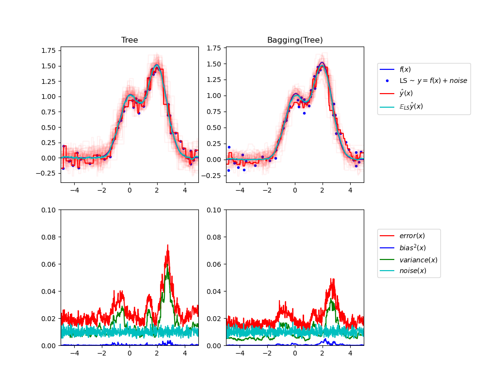
Ensemble methods, like the Random Forest you've used, are a powerful technique for managing this tradeoff. For example, Bagging (Bootstrap Aggregating) is designed specifically to reduce variance. It works by training many models on different subsets of the data and averaging their predictions.

This figure from `scikit-learn`'s documentation compares the error of a single Decision Tree (left) with a Bagging ensemble of Decision Trees (right). The single tree is a high-variance model, as shown by the large green `variance(x)` component. By averaging many trees, the Bagging model (right) dramatically reduces this variance, resulting in a lower, more stable total error (red curve).

Conclusion

In this lesson, we've dissected the fundamental challenge of building models that generalize. We've moved beyond the simple labels of "overfitting" and "underfitting" to the underlying causes: bias and variance.

Here are the key takeaways:

Bias is error from a model's simplifying assumptions, leading to underfitting.
Variance is error from a model's over-sensitivity to the training data, leading to overfitting.
The Bias-Variance Tradeoff is the core tension in modeling: decreasing one often increases the other. The goal is to find a balance that minimizes total error on unseen data.
Total Error is composed of $Bias^{2} + Variance + Irreducible Error$ . We can only influence the first two terms.
From an architect's standpoint, diagnosing whether a model suffers from high bias or high variance is the first step toward improving it.

You now possess the theoretical framework to understand why a model might be failing. In our next lesson, we will put this theory into practice. We will learn how to diagnose overfitting and underfitting using training and validation error curves, giving you the practical tools to see the bias-variance tradeoff in action with your own models.