Welcome to your second lesson. In our first session, we focused on the crucial task of problem framing—translating a high-level business objective into a concrete, solvable machine learning problem with clear success metrics. This is the strategic blueprint for any ML project. Now, having defined what we want to achieve, we must turn our attention to the primary raw material at our disposal: the data.
This lesson introduces Exploratory Data Analysis (EDA), the systematic process of investigating a dataset to understand its characteristics. From your perspective as an architect, you can think of EDA as performing due diligence on the foundational asset of your system. Just as you would inspect building materials for quality and suitability, EDA allows us to assess the quality, structure, and potential of our data. This process is not just about finding interesting patterns; it's about uncovering risks, identifying potential roadblocks, and gathering the necessary information to design a robust and reliable modeling pipeline.
By the end of this lesson, you will be able to perform exploratory data analysis to understand data types, distributions, and the relationships between variables, laying the groundwork for all subsequent feature engineering and modeling decisions.
What is Exploratory Data Analysis?
EDA is an approach to analyzing datasets to summarize their main characteristics, often with visual methods. Rather than testing a rigid hypothesis, the goal is to see what the data can tell us. It's about asking open-ended questions to generate hypotheses and guide the modeling process.
The following diagram provides a high-level overview of the key activities involved in EDA. It's a cycle of investigation that moves from understanding basic properties like central tendency and dispersion to visualizing relationships through graphical representations.
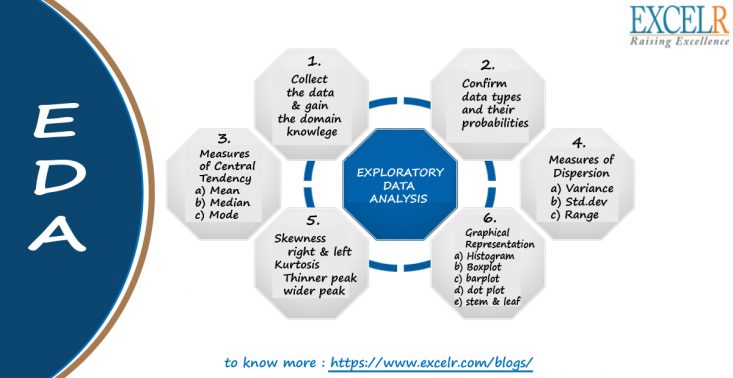
To formalize this, let's establish what EDA is, why it's essential, and what its concrete deliverables are. The following reading provides an excellent introduction.
Beginner's Guide to Exploratory Data Analysis
This guide from Georgia Tech's OMSCS program frames EDA as a systematic process with tangible outputs, which aligns well with an architect's need for documentation and process.
First, read the section "What Is Exploratory Data Analysis?" to understand its purpose and the key deliverables, such as a data dictionary and quality report. Then, jump to the end and read the conclusion starting from "By the End of EDA, You Should Have:". This list of outputs serves as a practical checklist for what you should aim to produce.
The Building Blocks: Data Types and Summary Statistics
A systematic exploration begins with understanding the most fundamental property of your data: its type. The type of a variable dictates the kinds of statistical summaries and visualizations that are appropriate. Your experience as a developer has made you familiar with data types in programming (e.g., int, string, float). In statistics, we use a slightly different, more descriptive categorization.
This next video offers a clear and concise explanation of the four main types of data in statistical analysis.
Professor Patrick Meyer provides a critical foundation for EDA by explaining the different scales of measurement. Understanding this is essential for choosing the correct analytical tools.
Watch the segment from the beginning until the end of the discussion on why data types matter. Pay close attention to the distinctions between nominal, ordinal, interval, and ratio data.
Once you know your data types, you can begin summarizing them using univariate analysis—looking at one variable at a time. This is typically done with non-graphical methods (summary statistics) and graphical methods (plots).
Non-Graphical Univariate Analysis
For any quantitative variable (interval or ratio data), we can describe its distribution using three key kinds of measures:
-
Central Tendency: This tells you about the "center" or "typical" value of the data.
- Mean: The arithmetic average. Sensitive to outliers.
- Median: The middle value (50th percentile). Robust to outliers.
- Mode: The most frequently occurring value.
-
Spread (or Variability): This describes how dispersed the data is around the center.
- Variance & Standard Deviation: Measures the average distance of data points from the mean.
- Interquartile Range (IQR): The range between the 25th (Q1) and 75th (Q3) percentiles. It captures the spread of the middle 50% of the data and is robust to outliers.
-
Shape: This characterizes the overall form of the distribution.
- Skewness: Measures the asymmetry of the distribution. A "tail" to the right indicates positive skew; a tail to the left indicates negative skew.
- Kurtosis: Measures the "tailedness" of the distribution. High kurtosis means more of the variance is due to infrequent extreme deviations (heavy tails), as opposed to frequent modest deviations.
The following reading from a Carnegie Mellon course provides detailed definitions for these essential statistics.
Chapter 4 Exploratory Data Analysis
This document offers a thorough, textbook-style explanation of the core statistical measures used in EDA. We'll focus on the sections that define the key terms for quantitative data.
Please navigate to section 4.2.2, "Characteristics of quantitative data." Read the subsections on Central tendency (4.2.3), Spread (4.2.4), and Skewness and kurtosis (4.2.5). Focus on understanding the definition and interpretation of each statistic, particularly the distinction between mean and median, and standard deviation and IQR.
Visualizing Data: From Numbers to Insights
While summary statistics are powerful, they can sometimes be misleading. Visualization is essential for building a true intuition for the data's structure.
Graphical Univariate Analysis
The most common tools for visualizing a single variable are:
- Histograms: These plots show the frequency distribution of a quantitative variable by grouping values into "bins." They are excellent for visualizing the shape, center, and spread of the data.
- Box Plots: These provide a compact summary of a quantitative variable based on its quartiles. A box plot clearly shows the median, the IQR (the box), and can be used to identify potential outliers—data points that fall unusually far from the rest of the data.
This image shows a collection of histograms for different features in a bank churn dataset. This is a typical output of a first-pass univariate analysis, allowing you to quickly scan the distributions of all your variables.

Bivariate and Multivariate Analysis
After understanding individual variables, the next step is to explore relationships between them.
- Scatter Plots: The standard tool for visualizing the relationship between two quantitative variables.
- Pair Plots: A powerful technique that creates a matrix of scatter plots for every pair of quantitative variables in your dataset, with histograms or density plots along the diagonal. This provides a comprehensive overview of all bivariate relationships.
- Correlation Heatmaps: A correlation matrix quantifies the linear relationship between pairs of variables. A heatmap visualizes this matrix with colors, making it easy to spot strong positive or negative correlations at a glance.
A Practical EDA Workflow with Python
Now, let's see how these concepts are applied in practice. Since you have experience with Python and scikit-learn, we'll look at a typical EDA workflow using the pandas, matplotlib, and seaborn libraries. This video provides a great hands-on demonstration.
Exploratory Data Analysis with Pandas Python
This video by Rob Mulla walks through a complete EDA process on a real-world dataset. It's an excellent demonstration of how to translate the statistical concepts we've discussed into code and visualizations.
First, watch the section on univariate analysis here. This shows how to generate value_counts for categorical data and histograms/KDE plots for continuous data. Next, watch the section on feature relationships here. This covers creating scatter plots, pair plots, and correlation heatmaps to explore how variables interact.
The workflow demonstrated in the video highlights a standard, repeatable process that you can adopt in your own projects:
- Initial Inspection: Check the data's shape, data types (
dtypes), and look at the first few rows (head). - Data Cleaning: Select relevant columns, handle missing values, and check for duplicates.
- Univariate Analysis: Analyze each feature individually using
.describe(),.value_counts(), histograms, and box plots. - Bivariate/Multivariate Analysis: Explore relationships between features using scatter plots, pair plots, and correlation matrices.
- Hypothesis Generation: Use the insights gained to ask deeper questions about the data, which can then be investigated further. For example, "How does the distribution of feature A differ across categories of feature B?"
This systematic approach ensures that you don't miss critical data characteristics and that your findings are reproducible, which is vital from an architectural standpoint.
Conclusion
In this lesson, we took our first deep dive into the data itself. We moved from the strategic exercise of problem framing to the tactical, hands-on process of Exploratory Data Analysis.
Here are the key takeaways:
- EDA is a Systematic Process: It's a crucial, open-ended investigation to understand your data's structure, identify quality issues, and uncover patterns.
- Know Your Data Types: The distinction between categorical (nominal, ordinal) and quantitative (interval, ratio) data determines which statistical summaries and visualizations are appropriate.
- Summarize and Visualize: Use a combination of summary statistics (mean, median, standard deviation, IQR) and visualizations (histograms, box plots, scatter plots) to build a comprehensive understanding of your data.
- From One to Many: Start with univariate analysis to understand individual variables, then move to bivariate and multivariate analysis to explore relationships between them.
You now have a framework and a set of tools to "interview" your data—to understand its story before you try to force it into a modeling narrative. The insights you gain here are invaluable. For instance, discovering a highly skewed feature might suggest the need for a logarithmic transformation. Identifying outliers will prompt a discussion on whether to remove them or use a robust model. Spotting a strong correlation between two features might influence your feature selection strategy.
In our next lesson, we will introduce a core concept in machine learning theory: the bias-variance tradeoff. The characteristics of your data, which you've learned to uncover through EDA, will have a direct and profound impact on where your models fall on this spectrum.