Hello! Welcome back to our course on Computerized Accounting.
In the last lesson, we defined what a Pivot Table is and discussed its powerful advantages for summarizing large datasets. You learned that it's an interactive report that can query, aggregate, and reformat data to answer business questions quickly.
Now, we will move from the "what" and "why" to the "how." This lesson is focused on a core practical skill and a very common exam question: outlining the steps to create a Pivot Table from a given dataset. By the end of this lesson, you will be able to confidently describe this multi-step process.
1. The Foundation: Preparing Your Data
Before you can create a Pivot Table, you must ensure your source data is structured correctly. This is the most critical step, as a poorly organized dataset will not work with a Pivot Table.
The data must be in a tabular format, which means:
- Each column must have a unique header (e.g., 'Date', 'Sales Amount', 'Region').
- There should be no blank rows or columns within your data.
- Each row should represent a single record or transaction.
To see why this is so important and learn a best-practice tip, watch the beginning of the following tutorial.
Pivot Table Excel | Step-by-Step Tutorial
In this video, Kevin Stratvert explains the importance of having data in a tabular format. He also demonstrates a highly recommended (though optional) step: converting your data range into an official Excel Table.
Watch from 00:10 to 00:50. Pay close attention to the definition of 'tabular format' and the process of inserting a Table using the 'Insert' tab. Converting to a table helps your Pivot Table update automatically when you add new data.
2. The Core Process: Creating a Pivot Table
Once your data is prepared, creating the Pivot Table involves a straightforward sequence of steps. We will break this down into two main phases: inserting the Pivot Table and building the report.
Step 1: Inserting the Pivot Table
This step creates the blank Pivot Table framework and opens the tool pane you will use to build your report.
Pivot Table Excel | Step-by-Step Tutorial
Continuing with the same video, let's see how to insert the Pivot Table itself.
Watch from 00:50 to 01:14. Notice the two main choices in the 'Create PivotTable' dialog box: the data source (your table) and the location for the report (a new or existing worksheet).
To summarize the insertion process:
- Click on any single cell inside your data table.
- Navigate to the Insert tab on the Excel ribbon.
- Click the PivotTable button.
- In the dialog box that appears, confirm that the correct table or range is selected.
- Choose whether to place the Pivot Table on a New Worksheet (recommended) or an Existing Worksheet.
- Click OK.
You will now have a blank Pivot Table on the left and a PivotTable Fields pane on the right side of your screen. This pane is your control center for building the report.
Step 2: Building the Report with the Field List
This is where you bring your report to life. The PivotTable Fields pane lists all the column headers from your source data. Below this list are four areas that represent the different parts of your report: Rows, Columns, Values, and Filters.
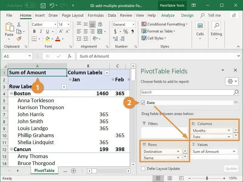
Here’s what each area does:
- Rows: Fields placed here will appear as row labels down the left side of the Pivot Table. (e.g., a list of Salespersons).
- Columns: Fields placed here will appear as column labels across the top. (e.g., different Product Categories).
- Values: This area is for the fields you want to calculate. It's almost always used for numerical data (e.g., 'Sales Amount'). By default, Excel will sum the numbers, but you can change this to count, average, max, min, etc.
- Filters: Fields placed here create a filter dropdown above the Pivot Table, allowing you to narrow down the entire report to specific data (e.g., filter all sales data by 'Year').
The following clips will demonstrate how dragging and dropping these fields instantly creates a summary report.
Pivot Table Excel | Step-by-Step Tutorial
This clip from Kevin Stratvert's tutorial shows the fundamental action of dragging fields to the 'Rows' and 'Values' areas to create a basic summary. It then shows how to add another layer of analysis using the 'Columns' area.
Please watch the following three segments: (01:14 - 02:48): Watch how dragging 'Salesperson' to Rows and 'Sales Amount' to Values creates an instant summary. (03:39 - 04:45): See how the 'Region' field is first added to Columns, and then moved to Rows to change the report's structure. (04:58 - 05:52): Observe how dragging 'Product' to the Filters area allows you to analyze the data for a specific product.
3. Summary of Steps for Your Exam
For a 6-mark question that asks you to outline the process, you need a clear, sequential answer. Your NCERT textbook and other resources provide a consistent set of steps.
Let's consolidate everything into a step-by-step guide you can use for revision.
Pivot Tables in Excel - GeeksforGeeks
The following article from GeeksforGeeks provides a very clear, step-by-step summary of the entire process. It's structured perfectly for an exam answer.
Read the section '1. Creating a Pivot Table in Excel'. Focus on the sub-headings from 'Step 1: Preparing the Data' through 'Step 4: Build our Pivot Table'. This provides a concise summary of the process.
Based on these resources, here is the process you should be able to outline:
- Prepare the Data: Ensure the data is in a clean tabular format with headers for each column and no blank rows or columns.
- Select the Data: Click any cell within the dataset.
- Insert the Pivot Table: Go to the
Inserttab and click onPivotTable. - Confirm Settings: In the 'Create PivotTable' dialog box, verify the data range and choose 'New Worksheet' as the location for the report. Click
OK. - Build the Report: A blank Pivot Table and a 'PivotTable Field List' will appear. Drag the required fields from the field list into the four areas:
- Drag descriptive fields (like 'Name' or 'Region') to the Rows or Columns areas.
- Drag numerical fields (like 'Sales' or 'Quantity') to the Values area to perform calculations.
- Drag fields you want to filter by (like 'Year' or 'City') to the Filters area.
The Pivot Table will automatically generate the summarized report based on your field placements.
Conclusion
You now have a complete, step-by-step guide to creating a Pivot Table. Mastering this procedure is not just about passing an exam; it's about learning one of the most powerful data analysis tools available in a spreadsheet.
Key Takeaways:
- Creating a Pivot Table starts with well-structured, tabular data.
- The process is initiated from the Insert > PivotTable menu.
- The core of building the report is dragging fields into the four key areas: Rows, Columns, Values, and Filters.
- Each area serves a distinct purpose in structuring and summarizing your data.
In our next lesson, we will build upon this foundation. Now that you know how to create a Pivot Table, you will learn how to filter and rearrange the data within an existing Pivot Table to answer even more specific analytical questions.