Hello! Welcome back to our course on Computerized Accounting.
In our previous lesson, you learned the essential steps to create a Pivot Table from raw data. You now know how to insert a Pivot Table and build a basic report by dragging fields into the Rows, Columns, and Values areas.
Today, we will unlock the true power of Pivot Tables by focusing on their interactive nature. The learning outcome for this lesson is to describe how to filter and rearrange data within a Pivot Table. Mastering these skills allows you to "slice and dice" your data to answer specific questions, a crucial skill for analysis and a frequent topic in your board exams.
1. Rearranging Data for New Perspectives
Once you've created a Pivot Table, you are not stuck with the initial layout. Rearranging, or "pivoting," is the core feature that gives the tool its name. It allows you to look at the same data from different angles to uncover new insights. There are three primary ways to rearrange data.
Method 1: Moving Fields Between Areas
The most fundamental way to rearrange your report is by moving fields between the four main areas of the PivotTable Fields pane (Rows, Columns, Values, Filters). For example, moving a field from the Rows area to the Columns area will completely change the report's orientation.

Let's watch a demonstration of this.
Pivot Table Excel | Step-by-Step Tutorial
This clip from the Kevin Stratvert tutorial we used previously shows how moving a field ('Region') from Columns to Rows instantly restructures the report.
Watch from 03:39 to 04:45. Notice how the report layout changes when the 'Region' field is moved from the Columns area to the Rows area. This is the essence of "pivoting" your data.
Method 2: Changing the Order of Fields
When you have multiple fields in one area (e.g., both 'Region' and 'Salesperson' in the Rows area), their order creates a hierarchy. The field on top is the primary grouping, and the one below it is the sub-grouping. Changing their order can significantly improve the clarity of your report.
The video segment you just watched (03:39 to 04:45) also demonstrates this. After moving 'Region' to the Rows area, you see how dragging it above 'Salesperson' changes the grouping from Salesperson -> Region to Region -> Salesperson.
You can also do this by using the dropdown menu on the field in the PivotTable Fields pane, as described in the Carnegie Mellon University PDF.
[PDF] advanced excel – vlookup, hlookup and pivot tables
This guide from Carnegie Mellon University provides a text-based explanation of how to reorder fields, which is useful for formulating exam answers.
Read the section titled 'Moving Fields' (pages 37-38). Focus on point 4, 'I may want my dollars summarized by Organization first then Object code.' It shows how to change the field order using the dropdown menu ('Move to Beginning').
Method 3: Sorting Data
Sorting allows you to rank your data, making it easy to spot top performers, best-selling items, or regions with the highest sales. You can sort labels alphabetically (A-Z or Z-A) or, more commonly, sort based on the values (largest to smallest or smallest to largest).
Pivot Table Excel | Step-by-Step Tutorial
This short clip demonstrates how to sort the data to quickly find the salesperson with the highest or lowest sales.
Watch from 03:14 to 03:50. Observe how right-clicking on a value cell gives you the 'Sort' option, allowing you to rearrange the data from 'Smallest to Largest' or 'Largest to Smallest'.
2. Filtering Data to Focus on Specifics
Filtering is the process of hiding data that is not relevant to your current question. This helps you focus on a specific subset of your information without deleting any of the underlying source data.
Method 1: The Report Filter
The Filters area in the PivotTable Fields pane is designed to apply a high-level filter to the entire report. When you place a field here (e.g., 'Year'), a dropdown menu appears above the Pivot Table, allowing you to view data for one, some, or all items in that field.
Pivot Table Excel | Step-by-Step Tutorial
Let's see the Report Filter in action. This clip shows how to filter the entire sales report by a specific product.
Watch from 04:58 to 05:52. Notice how dragging the 'Product' field to the 'Filters' area creates a dropdown menu above the table. Selecting 'Chocolate Chip' updates the entire Pivot Table to show data for only that product.
Method 2: Row/Column Label Filters and Advanced Filters
In addition to the main Report Filter, you can also filter directly using the dropdown arrows next to the 'Row Labels' and 'Column Labels' headers in the Pivot Table itself. These provide more granular filtering options.
For your exam preparation, it is useful to know the different types of filters available.
Introduction to Pivot Tables - Data Literacy for Students - EduRev
This article clearly outlines the various ways you can filter data in a Pivot Table. This is excellent material for structuring a detailed answer in an exam.
Read the section titled '3.6 Filtering Data in Pivot Tables'. Pay close attention to the definitions of 'Report Filter,' 'Row/Column Filters,' 'Value Filters,' and 'Top 10 Filter.' Understanding these different types will allow you to give a comprehensive answer.
As you read, you'll learn about:
- Row/Column Filters: Clicking the dropdown on a header to check/uncheck specific items to show or hide.
- Value Filters: Filtering based on the summarized values (e.g., show all regions with sales "greater than" 10,000).
- Top 10 Filter: A quick way to find top or bottom performers (e.g., "Top 5 Salespersons").
Method 3: Using Slicers
Slicers are a modern, highly visual, and user-friendly way to filter Pivot Tables. They are essentially interactive buttons that float on your worksheet, making it easy to see what you have filtered by.
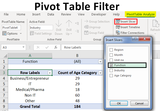
The following video shows how a slicer works once it's been inserted.
Pivot Table Excel | Step-by-Step Tutorial
This final clip demonstrates the power and simplicity of using slicers for interactive filtering.
Watch from 07:29 to 08:05. See how clicking on different regions in the slicer instantly filters the Pivot Table and an associated Pivot Chart. This is a powerful feature for creating interactive dashboards.
Conclusion
In this lesson, you've learned how to take a static Pivot Table report and turn it into a dynamic analysis tool. By mastering these techniques, you can answer complex business questions quickly and efficiently.
Key Takeaways:
- Rearranging Data: You can change the layout of your report by moving fields between areas, reordering fields within an area to change the grouping hierarchy, and sorting data to rank it.
- Filtering Data: You can focus on specific data subsets using the Report Filter, Row/Column label filters, or modern Slicers.
- Dynamic Analysis: All these actions are non-destructive. They simply change your view of the data, not the underlying source table.
This lesson concludes our module on data analysis and visualization in spreadsheets. You now have a solid understanding of charts and Pivot Tables, which are key components of the CBSE syllabus.
In our next lesson, we will move to the final module, Transaction Processing and Security. We will begin by exploring the fundamental building blocks of record-keeping in a Computerized Accounting System: the standard voucher types like Payment, Receipt, Sales, and Purchase.