Hello! Let's continue our exploration of data visualization in spreadsheets.
In our previous lesson, we familiarized ourselves with the anatomy of a chart, learning to identify and describe its key components like the data series, legend, and data labels. We learned what the parts are. Now, it's time to learn how to build the whole picture.
This lesson focuses on a very practical and frequently tested skill: outlining the steps to create a chart from a selected data range. By the end of this session, you'll be able to confidently describe this process, which is a common requirement in the CBSE exam.
1. The Starting Point: Preparing Your Data
Before a spreadsheet program can create a chart, it needs clean, well-organized data. This is the most crucial first step. For accounting purposes, this usually means having your data in columns with clear headings.
For example, you might have:
- A column for "Month" and a corresponding column for "Sales Amount".
- A column for "Expense Category" and a corresponding column for "Amount".
Once your data is ready, the creation process begins with selecting it.
Step 1: Select the Data Range
You need to tell the spreadsheet exactly what information to include in the chart.
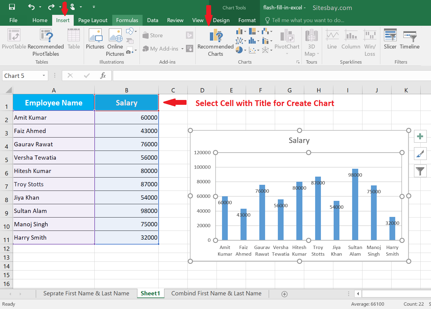
- Click and drag your mouse to highlight all the cells that contain the data you want to visualize.
- Crucially, make sure to include the column headers (e.g., "Month" and "Sales"). The spreadsheet uses these headers to automatically label the chart's axes and legend.
- An important tip: If your data includes a "Total" row, it's usually best to exclude it from your selection. Including the total can distort the scale of the chart and make it difficult to compare the individual data points.
2. From Data to Visual: The Creation Process
With your data selected, you are just a few clicks away from creating a chart. The process is straightforward and is managed from the Insert tab in most spreadsheet applications like Excel.
Video Walkthrough
The best way to learn these steps is to see them in action. The following video provides a clear, practical demonstration.
Excel Charts and Graphs Tutorial
This tutorial from Kevin Stratvert will walk you through the fundamental process of creating a chart. Pay close attention to how he selects the data, navigates to the 'Insert' tab, and chooses a chart type.
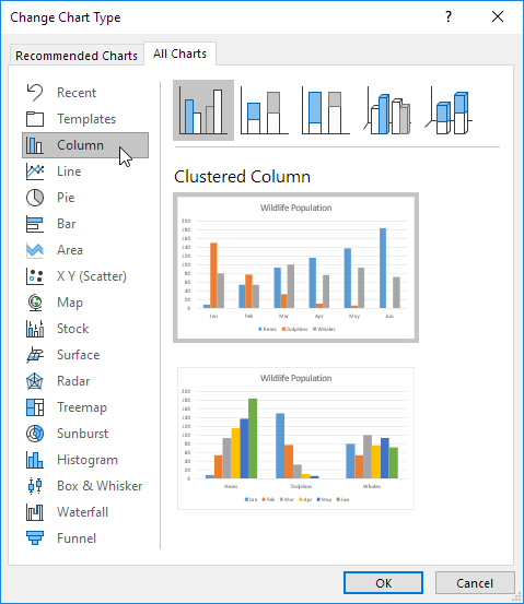
Please watch from 00:53 to 03:51. Focus on the sequence of actions: 1. Highlighting the data. 2. Clicking the 'Insert' tab. 3. Exploring 'Recommended Charts' and the 'All Charts' gallery to select a chart.
Textbook Steps for Exam Answers
The video showed you the practical process. Now, let's review these steps in a more formal way, just as you might need to write them in your exam. The following resource outlines the process clearly.
This PDF document provides a step-by-step guide to creating a chart, complete with illustrations. This format is perfect for memorizing the procedure for your exam.
Read section 5.22.1.3.1, titled 'CREATING A CHART / EMBEDDED CHART'. You can find this starting on page 5.90. It clearly lists the steps and shows corresponding images.
As you saw in both the video and the reading, a key step is choosing the right type of chart. While the software might recommend one, you should know the main types and their uses:
- Column/Bar Chart: Best for comparing values across different categories (e.g., sales by different salespeople).
- Line Chart: Ideal for showing trends over a period of time (e.g., monthly revenue over a year).
- Pie Chart: Used to show the proportion of individual parts to a whole (e.g., the percentage breakdown of total expenses by category).
3. A Concise Summary: The Steps to Create a Chart
For your exam, you may need to provide a concise, step-by-step answer. Based on what we've learned, here is a clear, five-step summary.
Write the step to create a bar chart in a spreadsheet.
This web resource provides an extremely clear and concise summary of the steps. It's a perfect model for how to structure your answer in an exam.
Read the 'Step by Step Solution' section. It breaks down the process into five simple, easy-to-remember steps.
To summarize, the essential steps are:
- Enter Data: Input your data into columns with clear headers.
- Select Data: Highlight the range of cells you want to chart, including the headers.
- Navigate to Insert: Click on the
Inserttab in the main menu. - Choose Chart: In the 'Charts' group, select the desired chart type (e.g., Column, Bar, Line).
- Insert Chart: The chart will be automatically created and placed on your worksheet.
Conclusion
Excellent work! You now have a solid understanding of the procedure for creating charts in a spreadsheet. You've seen it demonstrated, read the formal steps, and reviewed a concise summary perfect for exam preparation.
Key Takeaways:
- Chart creation always begins with well-organized and selected data.
- The core steps are: Select Data -> Insert Tab -> Choose Chart Type.
- It's important to include headers in your selection but exclude totals to avoid skewing the chart.
- Choosing the right chart type (Column, Line, Pie) depends on whether you want to compare values, show trends, or represent parts of a whole.
In the previous lesson, we identified the legend as a key chart element. In our next lesson, we will build on today's skill by learning how to reposition a legend on a chart, a common customization task that improves a chart's readability.