Arrays vs. Hash Maps: Choosing the Right Tool

Hello! In our last lesson, we explored string manipulation, specifically tackling palindrome and anagram problems. You saw a clear example of a performance trade-off when we compared solving the anagram problem by sorting versus using a hash map for frequency counting. This highlighted that choosing the right data structure is often the key to an optimal solution.

Today, we will build directly on that insight. This lesson is dedicated to formalizing the analysis and articulation of the trade-offs between two of the most fundamental data structures: arrays and hash maps. Mastering this comparison is not just about writing efficient code; it's about being able to justify your architectural decisions, a skill that is heavily scrutinized in top-tier technical interviews.

By the end of this lesson, you will be able to confidently choose between an array and a hash map for a given problem and clearly explain the time and space complexity implications of your choice.

The Array: A Model of Contiguous Memory

At its core, an array is a collection of items stored in a contiguous block of memory. This physical layout is the source of all its performance characteristics. Python's list is a dynamic array, which means it can grow in size, but the underlying principles are the same.

The most significant advantage of this contiguous storage is constant-time access by index.

Data Structure and Algorithm Patterns for LeetCode Interviews – Tutorial

This clip from a freeCodeCamp.org tutorial on data structure patterns explains the fundamental trade-offs of using arrays.

Watch the section on arrays. Pay close attention to the "row of houses" analogy, which explains why index-based access is O(1), and why insertions or deletions in the middle are expensive O(N) operations.

To summarize the key characteristics of an array (or Python list):

Access by index: $O (1)$ . You can jump directly to any element if you know its position.
Search by value: $O (N)$ . To find if an element exists, you may need to scan the entire array.
Insertion/Deletion at the end: Amortized $O (1)$ . Adding to the end is usually fast, but occasionally requires resizing the entire array, which averages out to constant time.
Insertion/Deletion at the beginning/middle: $O (N)$ . This requires shifting all subsequent elements, making it a costly operation for large arrays.

Arrays are the natural choice when the order of elements is critical and you need to perform sequential processing, such as with the two-pointer or sliding window patterns we've covered.

The Hash Map: The Key to Fast Lookups

Hash maps, known as dictionaries in Python, operate on a completely different principle. Instead of relying on a contiguous sequence, they use a hash function to map a key to an index in an underlying array, often called a bucket array.

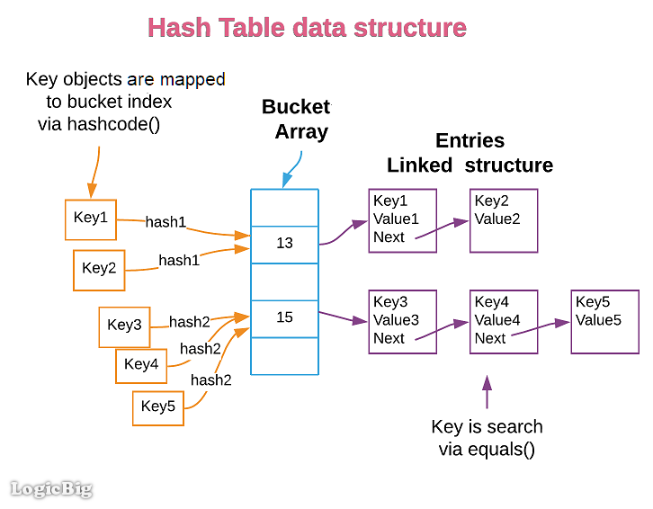
This diagram illustrates the core mechanism of a hash table. A hash function converts a key into an index in the "Bucket Array." To handle cases where different keys map to the same index (a "collision"), each bucket can hold a linked list of key-value pairs.

This mechanism allows hash maps to achieve their most famous feature: average-case $O (1)$ time complexity for lookups, insertions, and deletions.

To understand this better, let's explore the mechanics of hashing and how collisions are handled.

Hash Tables: Hash Functions, Sets, & Maps - DSA Course in Python Lecture 4

In this video, Greg Hogg provides a clear, step-by-step explanation of how hash tables are built, from the hash function to collision resolution.

First, watch the introductory part explaining hash functions and collisions. This will clarify how a key is turned into an index and what happens when multiple keys map to the same spot. Next, see how this structure is used to build hash sets and hash maps. The explanation of "amortized" or "on average" O(1) time is crucial for interviews.

A Critical Detail: Hashable Keys

A key constraint of hash maps is that keys must be immutable. This is because the hash function's output must be consistent. If the key's value could change after it's inserted, its hash would also change, and the hash map would no longer be able to find it. This is a subtle but vital concept.

Hash Tables: Hash Functions, Sets, & Maps - DSA Course in Python Lecture 4

This next segment from the same video by Greg Hogg explains exactly what makes a data type "hashable" and why mutable types like lists cannot be used as dictionary keys.

Watch the section discussing what is hashable. This is a frequent interview question and a common source of bugs for developers.

In Python, this means types like strings, numbers, and tuples can be dictionary keys, but lists and other dictionaries cannot.

A Head-to-Head Comparison

Now that we understand the internal workings, let's explicitly compare the performance characteristics. The following reading provides a concise yet comprehensive summary table and demonstrates the performance differences with Python code.

Difference between List and Dictionary in Python

This GeeksforGeeks article directly compares Python's list and dict data structures, providing complexity tables and performance benchmarks.

Start by reviewing the initial summary table. This gives a high-level overview. Next, carefully study the Space-Time Complexities section. The detailed table comparing operations like Search, Insertion, and Deletion is the core of this lesson. Also, examine the code examples; they provide empirical proof of the theoretical complexities. Finally, read the Key Observations, which summarize the trade-offs perfectly.

Let's distill the findings into a clear decision-making framework.

Feature / Operation	Array (Python List)	Hash Map (Python Dict)	When to Prefer It
Access	By index: $O (1)$	By key: Avg. $O (1)$	Array: For sequential access. Hash Map: For direct lookup without knowing position.
Search (for value/key)	By value: $O (N)$	For key: Avg. $O (1)$	Hash Map: Unbeatable for fast existence checks.
Insertion	End: Amortized $O (1)$ Middle: $O (N)$	Avg. $O (1)$	Hash Map: If you need to add elements frequently and order is secondary.
Deletion	By index: $O (N)$ By value: $O (N)$	By key: Avg. $O (1)$	Hash Map: For frequent, fast removal of items.
Data Ordering	Ordered by insertion	Insertion-ordered (Python 3.7+)	Array: When order is a primary requirement for the algorithm (e.g., sorting, binary search).
Space Complexity	Lower overhead	Higher overhead (stores keys + values)	Array: When memory is a primary constraint.

This graph illustrates the growth rates of common complexities. The $O(1)$ and $O(\log n)$ complexities of hash maps and binary search are vastly superior to the $O(n)$ or $O(n^2)$ complexities of linear scans or nested loops as input size increases.

Analyzing Problem Scenarios

Let's apply this framework to common interview patterns.

Scenario 1: Fast Lookups (e.g., Two Sum)

The Two Sum problem asks you to find two numbers in an array that add up to a target.

Brute-Force (Arrays): A nested loop that checks every pair of numbers. Time: $O (N^{2})$ .
Optimal (Hash Map): Iterate through the array once. For each element x, check if target - x exists in a hash map of previously seen numbers. This check is $O (1)$ . Time: $O (N)$ , Space: $O (N)$ .

This is the classic example of a space-time trade-off. We use $O (N)$ extra space for the hash map to reduce the time complexity from quadratic to linear. The mindset is to "remember" what you've seen to avoid re-computing.

Data Structure and Algorithm Patterns for LeetCode Interviews – Tutorial

The freeCodeCamp video revisits this concept and applies it to the Two Sum problem.

First, watch the segment on the mindset shift from brute force to using a hash map to remember answers. Then, see it in action with a detailed walkthrough of the Two Sum solution, including a complexity analysis.

Scenario 2: The Exception to the Rule (Bounded Key Space)

Sometimes, a hash map is overkill. In our last lesson on anagrams, we needed to count character frequencies for lowercase English letters.

Hash Map: {'a': 2, 'b': 1, ...}. Works perfectly.
Array as a Direct-Access Table: counts = [0] * 26. Use ord(char) - ord('a') to get an index from 0-25.

When the set of possible keys is small and bounded (like 26 letters, 128 ASCII characters, etc.), an array is often simpler, faster (no hash computation), and more memory-efficient. Recognizing this demonstrates a deeper level of understanding.

Hash Map Patterns That Show Up in Every Interview - CodeJeet

This article from CodeJeet discusses common hash map patterns and pitfalls.

Read the section on Common Pitfalls. Focus on the point about "Overusing hash maps" when a fixed-size array would be more efficient.

Articulating Your Choice in an Interview

Simply choosing the right data structure is not enough. You must communicate your thought process. Here’s a template:

Start with the naive solution. "My first thought is a brute-force approach. For the Two Sum problem, I could use nested loops to check every pair of numbers. This would give us a time complexity of $O (N^{2})$ and use $O (1)$ space."
Identify the bottleneck. "The bottleneck here is the inner loop, which performs an $O (N)$ scan to find the complement for each number. We're repeatedly searching for a value in an unsorted collection."
Propose the optimal data structure. "We can optimize this by trading space for time. If we use a hash map to store the numbers we've seen and their indices, we can reduce the lookup for the complement from $O (N)$ to an average of $O (1)$ ."
State the final complexity and trade-off. "By doing this, we iterate through the array only once. The overall time complexity becomes $O (N)$ , and we use $O (N)$ extra space for the hash map. This is a much better solution for large inputs."

Conclusion

Today we've systematically broken down the differences between arrays and hash maps, moving from their internal structure to their practical performance trade-offs. This analysis is central to algorithmic problem-solving.

Key Takeaways:

Arrays excel at ordered data and index-based access. Their contiguous memory layout makes sequential traversal fast but middle insertions/deletions slow.
Hash Maps excel at fast key-based lookups, insertions, and deletions. They achieve this via a hash function, at the cost of higher memory overhead and losing a strictly guaranteed order (though Python dictionaries maintain insertion order).
The core trade-off is often speed vs. memory. Hash maps frequently allow you to reduce time complexity (e.g., from $O (N^{2})$ to $O (N)$ ) by using extra space.
Articulating these trade-offs is as important as implementing the solution correctly in an interview setting.

This lesson concludes our module on Hashing, Arrays, and Strings. You are now equipped to handle a vast range of problems that rely on these fundamental tools. In our next module, we will introduce a new category of data structures—Linear Structures—starting with Linked Lists, which offer a completely different set of trade-offs compared to arrays.

Recommended resources