Merge Sort: Analyzing O(n log n) Complexity

1. Breaking Down O(n log n)

The O(n log n) complexity isn't arbitrary; it comes directly from the two main phases of the algorithm:

1. The log n part: This arises from the recursive "divide" step.
2. The n part: This comes from the "combine" step, where we merge the sorted halves.

Let's investigate each part, starting with log n.

The log n Component: The Depth of Recursion

The "divide" step of Merge Sort repeatedly splits the input list in half. The number of times you can halve a list of size n until you get down to lists of size 1 is precisely log₂(n).

To build a strong intuition for this, let's first consider a different problem.

As the article explains, repeatedly cutting the problem in half is a logarithmic process. Merge Sort does exactly this. An array of 8 elements is split into two arrays of 4, which are split into four arrays of 2, which are finally split into eight arrays of 1. This took 3 levels of splits, and log₂(8) = 3.

This means the depth of our recursion tree is log n.

The n Component: The Work at Each Level

Now, where does the n come from? It represents the work done in the "combine" or merge phase.

Recall the merge function you wrote. It takes two sorted sub-lists and combines them into one. To do this, it must look at every element in both sub-lists exactly once. Therefore, merging two lists with a total of k elements takes O(k) time.

The key insight for Merge Sort's analysis is that at every level of recursion, the total work done by merging adds up to O(n).

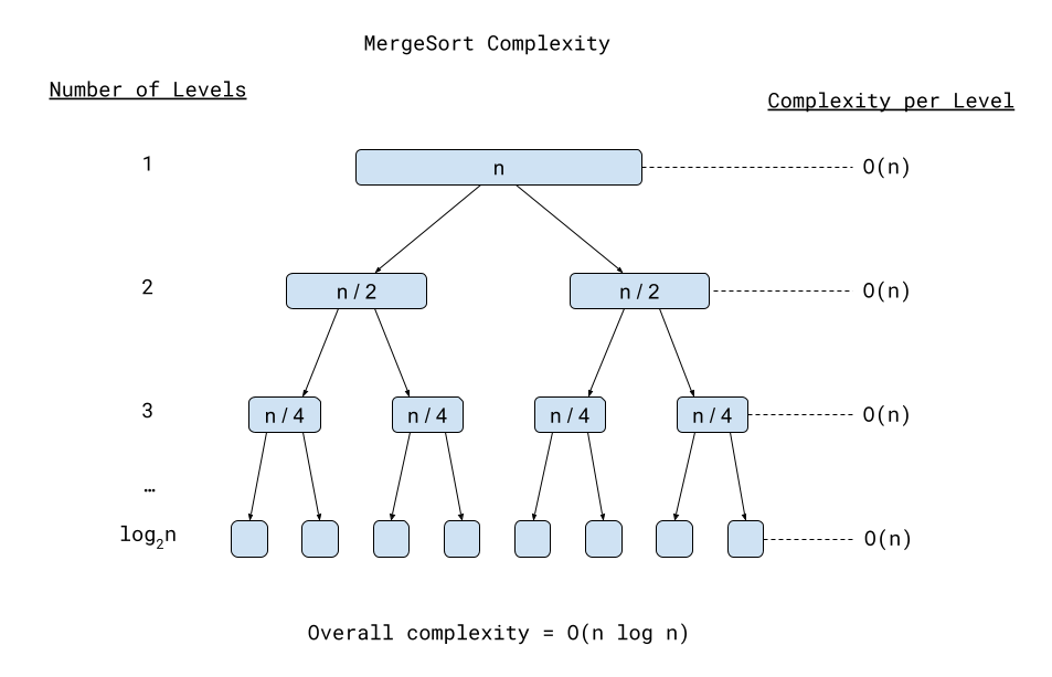
Let's visualize this:

• Level 1 (Top): We merge two lists of size n/2. Total elements merged: n/2 + n/2 = n. Work: O(n).
• Level 2: We perform two separate merges, each on lists of size n/4. Total elements merged: (n/4 + n/4) + (n/4 + n/4) = n. Work: O(n).
• Bottom Level: We perform n/2 merges, each on lists of size 1. Total elements merged: n/2 * (1 + 1) = n. Work: O(n).

No matter which level you're on, the total number of elements being processed across all merges is n.

This video provides a fantastic visualization of this concept.

2. Putting It All Together: log n Levels of n Work

Now we can combine our two findings:

• The algorithm creates O(log n) levels of recursive calls.
• At each level, it performs a total of O(n) work to merge the sub-lists.

Total Time = (Number of Levels) × (Work per Level)
$\text{Time Complexity}=O(\log n)\times O(n)=O(n\log n)$

This diagram perfectly summarizes the analysis:

3. A Formal Analysis: The Recurrence Relation

We can express the time complexity of a recursive algorithm like Merge Sort using a recurrence relation. This is a more formal, mathematical way to represent the work being done, which will be very useful as you analyze more complex algorithms.

Let T(n) be the time it takes to sort a list of n elements. We can define T(n) as follows:
$T(n)=\underset{\text{Conquer}}{\underbrace{2T(n/2)}}+\underset{\text{Combine}}{\underbrace{O(n)}}$

Let's break this down:

• T(n): The time to solve a problem of size n.
• 2T(n/2): The time to solve two recursive subproblems, each on a list of size n/2. This is the "Conquer" step where we call merge_sort on the left and right halves.
• O(n): The time to combine the results of the subproblems. This is the merge function, which we know takes linear time.

To solve this recurrence and show that it equals O(n log n), we can use a method called repeated substitution. This involves expanding the T(n/2) term repeatedly until we find a general pattern.

The following video provides an excellent walkthrough of this mathematical derivation. Since you're comfortable with algebra and logarithms, this method should feel quite intuitive.

By following the substitution, you can see mathematically how the n term gets added at each of the log n levels of recursion, leading directly to the n log n result plus a lower-order n term, which we drop in Big O notation.

Conclusion

In this lesson, you've moved beyond simply knowing Merge Sort's complexity to understanding why it is O(n log n). This analytical skill is fundamental to algorithm design and a key part of technical interviews.

Key Takeaways:

• Merge Sort's time complexity is O(n log n) in all cases (best, average, and worst) because the division and merging steps are not dependent on the input data's order.
• The log n component comes from the number of times the list can be recursively halved—the depth of the recursion tree.
• The n component comes from the linear-time merge operation, as the total work done at each level of recursion is O(n).
• The formal way to express this is with the recurrence relation T(n) = 2T(n/2) + O(n), which can be solved to prove the O(n log n) complexity.

Preview of the Next Lesson:
Now that you have analyzed two sorting algorithms with very different efficiencies (Insertion Sort's O(n²), Merge Sort's O(n log n)), we are ready to take a broader look. In the next lesson, we will compare the performance trade-offs of different sorting algorithms, discussing when you might choose one over the other based on factors like input size, memory usage, and stability.