Divide and Conquer Strategy

1. The Core Idea: Break It Down

At its heart, divide and conquer is about making a large, overwhelming problem manageable by breaking it into smaller, identical problems.

To get a solid grasp of this concept, start by reading the first few sections of the following article. It provides a clear definition, a fantastic real-world analogy, and outlines the three distinct phases of the strategy.

2. The Three Phases of Divide and Conquer

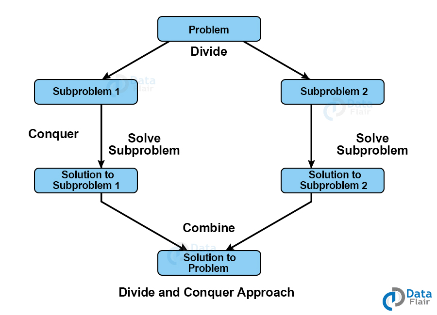
As you just read, every divide and conquer algorithm follows a consistent, three-step pattern:

1. Divide: Break the main problem into several smaller, independent subproblems. The crucial detail here is that the subproblems are just smaller instances of the original problem.
2. Conquer: Solve the subproblems. If the subproblems are still large, this step is applied recursively. This process continues until the subproblems become so small that they can be solved directly. This "small enough" version is called the base case.
3. Combine: Merge the solutions of the subproblems back together to form the solution for the original, larger problem.

This flow is captured perfectly in the following diagram:

3. The Recursive Nature of the Strategy

The "Conquer" step, where we recursively solve subproblems, is the engine of this strategy. It’s what makes divide and conquer so elegant and powerful. A key requirement is that the subproblems must be of the same type as the original. You can't divide a sorting problem into a set of searching problems.

This video explains this requirement very clearly and introduces the general, recursive structure of a divide and conquer algorithm.

Based on this, we can outline a general template for any divide and conquer algorithm. You can think of it like a function that calls itself:

function divide_and_conquer(problem P):
  // Base Case: If the problem is small enough, solve it directly.
  if P is small:
    return solve(P)
  
  // Recursive Step:
  else:
    // 1. Divide
    Divide P into subproblems P1, P2, ..., Pk

    // 2. Conquer
    solution1 = divide_and_conquer(P1)
    solution2 = divide_and_conquer(P2)
    ...

    // 3. Combine
    result = combine(solution1, solution2, ...)
    return result

This structure might remind you of mathematical induction, where you prove a base case and then an inductive step that relies on the assumption that the statement holds for smaller cases.

4. Divide and Conquer in Action: Examples

Let's see how this pattern applies to algorithms you know and algorithms you're about to learn.

Binary Search (A Degenerate Case)
We can re-frame the binary search algorithm we learned previously:

• Divide: "Divide" the array by finding the middle element.
• Conquer: Compare the target to the middle element. This solves the problem for the middle element and tells you which subproblem (the left or right half) to solve next.
• Combine: There is no combination step! The solution to one of the subproblems is the final answer. This is a common pattern for search-style problems.

Merge Sort (A Classic Case)
This is a powerful sorting algorithm that we will implement in the next lesson. It follows the divide and conquer pattern perfectly:

• Divide: Split the unsorted list into two equal halves.
• Conquer: Recursively call merge sort on each of the two halves. The recursion stops when a sub-list has only one element (the base case), as a list of one is already sorted.
• Combine: Merge the two sorted sub-lists back into one single, sorted list. This "merge" step is the most important part of the algorithm.

5. Advantages and Disadvantages

So, why go through the trouble of this recursive approach? The primary reason is efficiency. By breaking problems down, we can often achieve significantly better time complexities. However, it's not a silver bullet for every problem.

The following article provides a concise summary of the pros and cons.

Here's a summary of the key points you just read:

• Advantages:

  • Efficiency: Often leads to very fast algorithms, like O(log n) or O(n log n), which are massive improvements over O(n²).
  • Solves Difficult Problems: Makes complex problems, like sorting, conceptually easier to tackle.
  • Parallelism: The independent subproblems can often be solved simultaneously on multi-core processors, further speeding up computation.

• Disadvantages:

  • Recursion Overhead: Recursive function calls use memory on the "call stack" and can be slightly slower than a simple loop for small problems.
  • Implementation Complexity: Can sometimes be harder to implement correctly than a straightforward iterative approach.

For large datasets, the efficiency gains from divide and conquer almost always outweigh the disadvantages.

Conclusion

Excellent work! You have now formally defined and explored one of the most important design paradigms in all of computer science. This strategy is a cornerstone of efficient problem-solving and will appear again and again in your study of algorithms.

Key Takeaways:

• The divide and conquer strategy consists of three steps: Divide, Conquer, and Combine.
• It works by recursively breaking a problem down into smaller, identical subproblems until they reach a base case that can be solved directly.
• The solutions to the subproblems are then merged to solve the original problem.
• This approach is the key to many highly efficient algorithms and is particularly effective for tasks that can be broken into independent parts.

Preview of the Next Lesson:
With this theoretical foundation in place, we are ready to get our hands dirty. In the next lesson, we will implement Merge Sort, our first divide and conquer sorting algorithm. You will write the code that brings this strategy to life and see firsthand how it achieves its impressive O(n log n) time complexity, leaving O(n²) algorithms like insertion sort far behind.