Introduction
Hello! In our last few lessons, we've taken a deep dive into specific sorting algorithms. You've implemented insertion sort and analyzed its O(n²) complexity, and you've implemented and analyzed merge sort, understanding why it achieves a much more efficient O(n log n) time complexity.
Today, we'll zoom out and look at the bigger picture. In a technical interview, knowing how to implement an algorithm is only half the battle. The other half is being able to justify your choice of algorithm by explaining its trade-offs. This lesson is dedicated to that skill: we will compare the performance trade-offs of different sorting algorithms.
We will move beyond just time complexity and consider other critical factors:
- Space Complexity: How much extra memory does the algorithm need?
- Stability: Does the algorithm preserve the original order of equal elements?
- Performance in different scenarios: How does the algorithm behave with nearly-sorted data or small inputs?
By the end of this lesson, you'll have a framework for deciding which sorting algorithm is the right tool for a given job.
1. The Landscape of Complexity
Let's start with a quick visual recap. The reason we prefer an O(n log n) algorithm over an O(n²) one for large datasets becomes obvious when you see their growth rates.
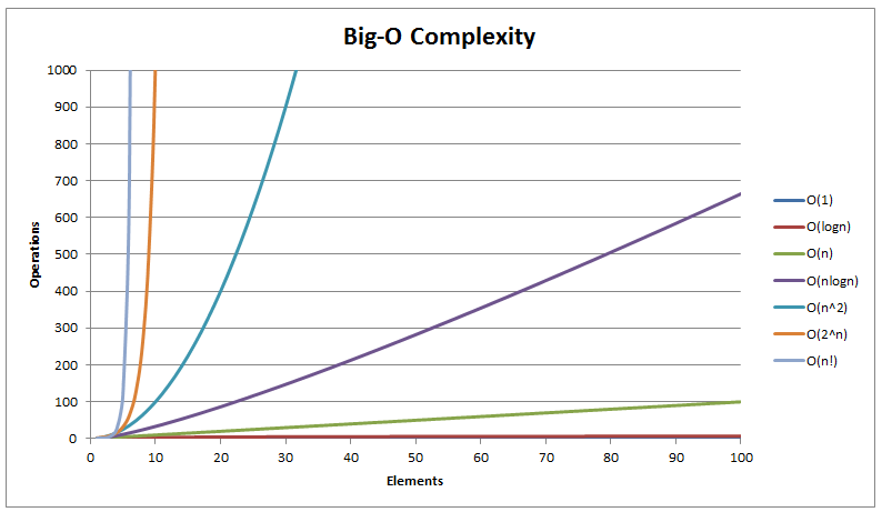
While O(n log n) is our theoretical goal for general-purpose sorting, we'll see that practical considerations can sometimes lead us to choose a different path.
2. A New Contender: Quicksort
You are now very familiar with Merge Sort, a "divide and conquer" algorithm. Let's introduce its famous cousin, Quicksort. Quicksort is also a divide and conquer algorithm and has an average time complexity of O(n log n). However, it approaches the problem differently, which leads to a crucial trade-off.
Instead of splitting the list in half and merging, Quicksort picks an element as a pivot and partitions the other elements into two sub-arrays, according to whether they are less than or greater than the pivot. It then recursively sorts the sub-arrays.
The key advantage? Quicksort can do this in-place, without creating large temporary copies of the arrays.
Let's watch a breakdown of Quicksort. Pay close attention to how it sorts the list without creating new arrays, which is its main advantage over Merge Sort.
Watch the section from 06:47 to 10:25. The video explains the partitioning process and highlights that Quicksort works 'in-place'. It also introduces Quicksort's 'dark side': a potential O(n²) worst-case performance if the pivot selection is poor.
As you saw, Quicksort's in-place nature is a huge win for memory efficiency. However, the choice of pivot is critical. A bad pivot (e.g., consistently picking the smallest or largest element) can unbalance the partitions and degrade its performance to O(n²). In practice, using a random pivot or the median-of-three elements largely prevents this worst-case scenario.
3. The Great Debate: Merge Sort vs. Quicksort
This is a classic technical interview topic. Both are O(n log n) on average, so which one should you choose? It depends entirely on the trade-offs you're willing to make.
| Feature | Merge Sort | Quicksort |
|---|---|---|
| Time (Avg) | O(n log n) |
O(n log n) (often faster in practice) |
| Time (Worst) | O(n log n) |
O(n²) |
| Space | O(n) |
O(log n) |
| Stability | Stable | Not Stable |
Let's unpack the most important differences: Space and Stability.
Space Complexity: O(n) vs. O(log n)
Merge Sort requires O(n) auxiliary space because the merge step needs a temporary array to combine the sorted halves.
Quicksort is considered an in-place algorithm, but it's not quite O(1) space. Because it's recursive, it uses space on the call stack to keep track of the recursive function calls. In the average case, the depth of this recursion is log n.
Sorting Algorithms Time and Space Complexity | Sorting Algorithms | Big-O | Geekific
This video clearly explains the difference in space requirements for Merge Sort and Quicksort.
Watch from 12:12 to 13:37. The narrator explains why Merge Sort's space complexity is O(n) (due to temporary arrays) while Quicksort's is O(log n) (due to the recursive call stack).
Trade-off: If memory is highly constrained, Quicksort's O(log n) space usage is a significant advantage over Merge Sort's O(n).
Stability
This is a new concept for us. A sorting algorithm is stable if it maintains the relative order of records with equal values.
Imagine sorting a spreadsheet of students first by name (alphabetically), and then by grade (numerically). If two students have the same grade, say 85%, a stable sort would ensure they remain in their original alphabetical order. An unstable sort might swap them.
Comparison of Sorting Algorithms
The concept of stability is crucial for certain applications. This article provides a clear definition and lists which common algorithms are stable.
Read the short section titled 'Stable sorting algorithms'. It defines stability and gives examples. Note that Merge Sort is stable, while Quicksort is not.
Trade-off: If you need to preserve the original order of equal elements, Merge Sort is the superior choice. If all elements are unique or their relative order doesn't matter, this factor is irrelevant.
4. When Are "Slow" Algorithms Useful?
With O(n log n) algorithms available, is there ever a reason to use an O(n²) algorithm like Insertion Sort? Absolutely.
Big O notation describes performance as n becomes very large. For small n, the simpler logic and lower overhead of Insertion Sort can actually make it faster than the more complex setup of Merge Sort or Quicksort.
Furthermore, Insertion Sort has an excellent best-case performance of O(n) when the data is already or nearly sorted.
Let's revisit Insertion Sort to see its specific niche.
Watch the section from 04:47 to 05:20. The video explains that Insertion Sort is highly effective on small datasets or data that is already mostly sorted.
This property is so useful that many professional-grade sorting implementations (like Python's built-in sort()) are hybrid algorithms. They use an algorithm like Merge Sort to break the list down into smaller chunks, then switch to Insertion Sort to finish the job on those small, manageable sub-lists.
5. A Decision-Making Framework
You're in an interview. You're asked to sort a large dataset. How do you decide which algorithm to use? You should think through a checklist of questions.
The following guide, based on the EnjoyAlgorithms article, provides an excellent framework for making this decision.
Comparison of Sorting Algorithms
This article provides a fantastic summary of how to select the right algorithm based on different constraints. We will use it as our guide.
Read the section 'How to choose the best sorting algorithm?'. This provides a checklist of factors to consider, which we will summarize below.
Here is a summary of the key questions to ask yourself:
- Is memory a major constraint?
- Yes: Prefer an in-place algorithm like Quicksort (
O(log n)space) or Heapsort (O(1)space - we haven't covered this, but it's good to know it exists). Avoid Merge Sort (O(n)space).
- Yes: Prefer an in-place algorithm like Quicksort (
- Is a guaranteed
O(n log n)worst-case time essential?- Yes: Use Merge Sort or Heapsort. Avoid Quicksort, whose worst-case is
O(n²). This is critical for real-time systems where performance predictability is key.
- Yes: Use Merge Sort or Heapsort. Avoid Quicksort, whose worst-case is
- Is the data nearly sorted?
- Yes: Insertion Sort is an excellent choice, as its performance approaches
O(n).
- Yes: Insertion Sort is an excellent choice, as its performance approaches
- Is the dataset small?
- Yes: The overhead of complex algorithms isn't worth it. Insertion Sort is often the fastest.
- Do you need to preserve the relative order of equal elements (stability)?
- Yes: Use a stable algorithm like Merge Sort or Insertion Sort. Avoid Quicksort and Heapsort.
In many general-purpose scenarios where memory is not extremely limited and the worst-case is unlikely, Quicksort is often chosen because its inner loop is very efficient, making it one of the fastest algorithms in practice on average.
Conclusion
Today, you've learned that choosing a sorting algorithm is a nuanced decision that involves analyzing trade-offs. There is no single "best" algorithm; the right choice depends on the specific constraints of the problem. Being able to articulate this analysis is a sign of a strong algorithmic thinker and will impress in technical interviews.
Key Takeaways:
- Merge Sort vs. Quicksort is the primary trade-off for large datasets. You're balancing Merge Sort's guaranteed
O(n log n)time and stability against Quicksort'sO(log n)space efficiency and often faster average-case speed. - Insertion Sort is not useless. It excels on small or nearly-sorted datasets and is a key component of many real-world hybrid sorting algorithms.
- Your decision-making process should always consider Time Complexity (Worst/Average), Space Complexity, and Stability.
Preview of the Next Lesson:
We've now concluded our deep dive into sorting algorithms. In the next module, we'll begin exploring a new category of data structures: Linear Data Structures. We'll start with the Stack, a simple but powerful Last-In, First-Out (LIFO) structure. You've already seen a practical example of a stack in action—the call stack that manages recursive calls in algorithms like Merge Sort and Quicksort! We'll now learn how to build and use them ourselves.