Graph Traversal with BFS and Queues

What is Breadth-First Search?

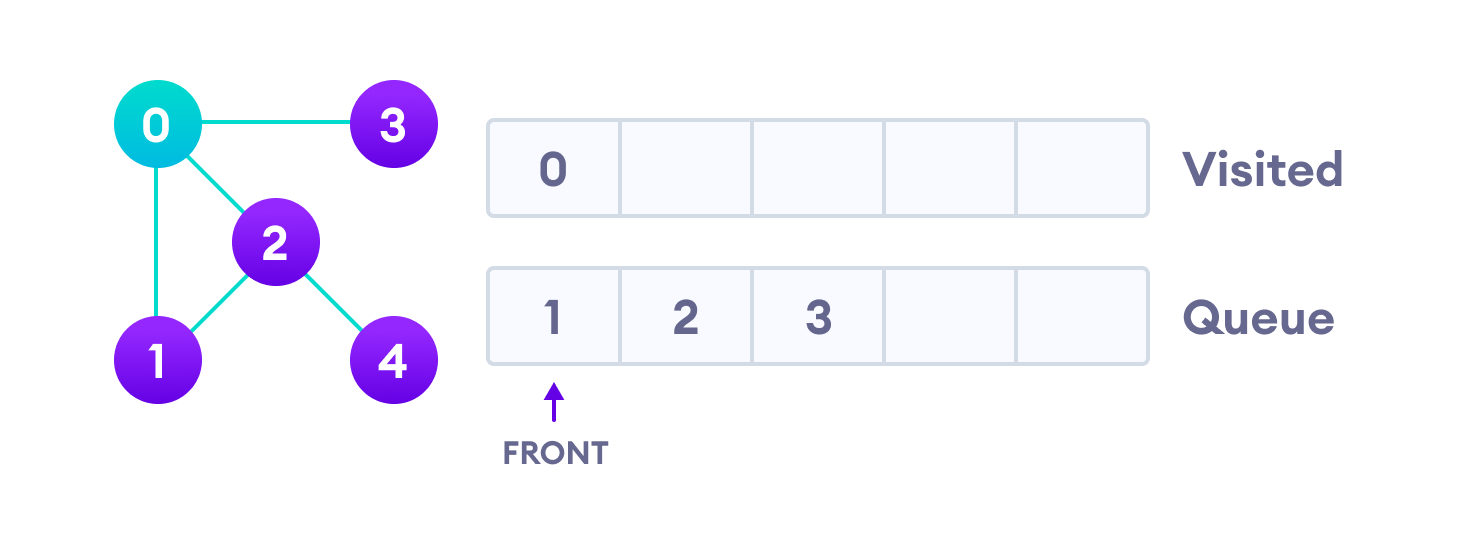
Breadth-First Search (BFS) is an algorithm for traversing a graph. It starts at a chosen "source" vertex and explores all of its immediate neighbors. Then, for each of those neighbors, it explores their unvisited neighbors, and so on, until all reachable vertices have been visited.

This level-by-level exploration has an important property: in an unweighted graph, the first time BFS reaches a vertex, it has found the shortest path (in terms of the number of edges) from the source to that vertex.

To visualize how BFS works, we'll watch a short, animated explanation. Pay close attention to the two key data structures it uses: a queue to manage which node to visit next, and a visited set to keep track of nodes we've already seen.

As you saw, the algorithm relies on three components:

1. The Graph: Represented as an adjacency list, just as we learned in the previous lesson.
2. A Queue: To store the vertices that are waiting to be explored. The FIFO (First-In, First-Out) nature of the queue is what ensures we explore level by level.
3. A Visited Set: To keep track of the vertices we have already visited. This is essential to avoid processing the same vertex multiple times and to prevent getting caught in an infinite loop if the graph contains cycles.

The BFS Algorithm Step-by-Step

Let's formalize the process you saw in the video into a clear, step-by-step algorithm.

Imagine we have a graph and a starting vertex.

1. Initialization:

   • Create a queue and add the starting vertex to it.
   • Create a visited set to store vertices we've already seen. Add the starting vertex to this set.

2. Exploration Loop:

   • While the queue is not empty, do the following:
     a. Dequeue: Remove the vertex from the front of the queue. Let's call it current_vertex.
     b. Process: Do something with current_vertex (e.g., print its value).
     c. Enqueue Neighbors: Look at the neighbors of current_vertex from our adjacency list. For each neighbor:
     i. If the neighbor is not in the visited set:
     - Add the neighbor to the visited set.
     - Add the neighbor to the back of the queue.

3. End:

   • Once the queue is empty, it means we have visited every vertex reachable from the starting vertex. The algorithm terminates.

Implementing BFS in Python

Now, let's translate this algorithm into Python code. This is where your knowledge from previous lessons on functions, loops, and data structures comes together.

We will use the adjacency list representation from our last lesson. For the queue, we'll use collections.deque, which is a highly efficient double-ended queue. While you can use a Python list, removing items from the front with list.pop(0) is slow. deque.popleft() is much faster, a detail that's important in a technical interview context.

Let's look at a complete implementation. The following code defines a graph and then implements the BFS function exactly as described.

# First, we need to import deque from the collections module
from collections import deque




# We'll use the graph representation from the Educative.io article
graph = {
  'A' : ['B','C'],
  'B' : ['D', 'E'],
  'C' : ['F'],
  'D' : [],
  'E' : ['F'],
  'F' : []
}

def bfs(graph, start_node):
    """
    Performs a Breadth-First Search on a graph.

    Args:
        graph (dict): The graph represented as an adjacency list.
        start_node (str): The node to start the traversal from.
    """



    # 1. Initialization
    visited = set()       # A set to keep track of visited nodes.
    queue = deque([start_node]) # A queue for nodes to visit, starting with the start_node.
    visited.add(start_node)




    # 2. Exploration Loop
    while queue:



        # a. Dequeue a vertex from the front of the queue
        current_node = queue.popleft()
        print(current_node, end=" ") # b. Process the node (in this case, print it)




        # c. Enqueue all unvisited neighbors
        for neighbor in graph[current_node]:
            if neighbor not in visited:
                visited.add(neighbor)   # Mark neighbor as visited
                queue.append(neighbor)  # Add neighbor to the queue




# Let's run the BFS starting from node 'A'
print("BFS traversal starting from node A:")
bfs(graph, 'A')

When you run this code, the output will be:
BFS traversal starting from node A:
A B C D E F

This order perfectly reflects the level-by-level traversal:

• Level 0: A
• Level 1: B, C
• Level 2: D, E, F

Practice Tracing

To solidify your understanding, try to trace the BFS algorithm yourself on a piece of paper.
Given the following graph and starting at node 0:

graph = {
    0: [1, 2],
    1: [2],
    2: [0, 3],
    3: [3]
}

Track the following:

1. The queue at the beginning of each loop iteration.
2. The visited set as it grows.
3. The final output (the order nodes are printed).

Conclusion

Congratulations! You have now learned and implemented your first graph traversal algorithm. BFS is a powerful tool with many applications, from finding shortest paths in games and networks to web crawlers indexing the internet.

Key Takeaways:

• Breadth-First Search (BFS) explores a graph level by level.
• It relies on a queue to maintain a First-In, First-Out order of exploration.
• A visited set is crucial to avoid redundant work and infinite loops in graphs with cycles.
• The most efficient way to implement the queue in Python is with collections.deque.
• The BFS algorithm is a direct application of the data structures we've learned, using an adjacency list as input.

Preview of the Next Lesson:

BFS is not the only way to traverse a graph. What if instead of exploring widely, we wanted to explore as deeply as possible along one path before backtracking? This alternative strategy is called Depth-First Search (DFS). In the next lesson, we will implement DFS using recursion and compare its behavior and use cases to BFS.