BFS for Shortest Paths in Unweighted Graphs

Why BFS is Perfect for Finding the Shortest Path

In an unweighted graph, the "cost" or "length" of a path is simply the number of edges it contains. The "shortest path" is therefore the path with the minimum number of edges.

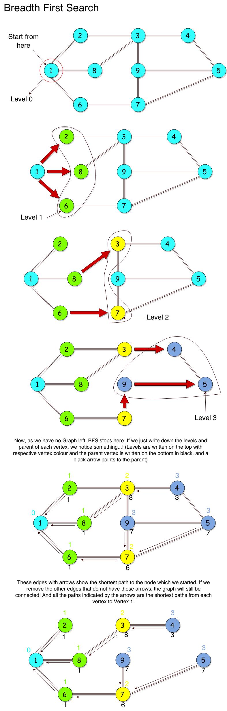
The reason BFS is guaranteed to find this shortest path is because of its very nature. It explores the graph in expanding layers of distance from the starting node:

• First, it visits all nodes at distance 1 (direct neighbors).
• Then, it visits all nodes at distance 2.
• Then, all nodes at distance 3, and so on.

Because of this orderly, layer-by-layer exploration, the first time BFS reaches a target node, it is guaranteed to have done so via the shortest possible path. Any other path would have to be longer or of the same length.

Let's watch a short video that provides a great analogy to help this concept click.

As the video explains, this property makes BFS the go-to method for shortest path problems in unweighted graphs.

Modifying BFS to Track Paths

Our standard BFS traversal algorithm is great at visiting nodes, but it doesn't inherently keep track of the paths taken. To find the shortest path, we need to add a mechanism to record how we reached each node.

We can achieve this by using a parent dictionary (sometimes called a predecessor map). This dictionary will store, for each node we visit, the node that led us to it.

parent = { 'B': 'A', 'C': 'A', 'D': 'B', ... }

This entry 'B': 'A' means "we discovered node 'B' via node 'A'".

Once BFS has found the target node, we can reconstruct the path by working backward from the target to the start using this parent dictionary.

Let's see how this works in practice.

To summarize the key ideas from the video:

1. Central Data Structure: We still use a queue for the main traversal, just like in standard BFS.
2. Tracking mechanism: We use a parent dictionary where parent[node] = previous_node. The start node's parent can be set to None.
3. Path Reconstruction: Once the target is found, we start from the target, look up its parent, then look up that node's parent, and so on, until we reach the start node (whose parent is None). This gives us the path in reverse order, which we then simply reverse to get the final result.

Python Implementation

Now let's translate this logic into a Python function. We will build upon the BFS traversal code you've seen before, adding the parent dictionary and the path reconstruction logic.

The following article provides a clean and complete implementation.

Here is the complete function, combining the pieces from the article. Take a moment to read through it and see how the concepts we've discussed come together.

from collections import deque

def find_shortest_path(graph, start, target):
    """
    Finds the shortest path between a start and target node in an unweighted graph using BFS.

    Args:
        graph (dict): The graph represented as an adjacency list.
        start: The starting node.
        target: The target node.

    Returns:
        A list representing the shortest path, or None if no path exists.
    """



    # A queue for the nodes to visit
    queue = deque([start])



    # A set to keep track of visited nodes to avoid cycles and redundant work
    visited = {start}



    # A dictionary to store the parent of each node to reconstruct the path
    parent = {start: None}

    while queue:
        current_node = queue.popleft()




        # If we found the target, we can stop and build the path
        if current_node == target:
            path = []



            # Backtrack from target to start using the parent dictionary
            while current_node is not None:
                path.append(current_node)
                current_node = parent[current_node]



            # The path is from target to start, so we reverse it
            return path[::-1]




        # Explore neighbors
        for neighbor in graph.get(current_node, []):
            if neighbor not in visited:
                visited.add(neighbor)



                # Record that we reached this neighbor from the current_node
                parent[neighbor] = current_node
                queue.append(neighbor)




    # If the queue becomes empty and we haven't found the target, there is no path
    return None




# --- Example Usage ---
# Let's use a simple graph to test
my_graph = {
    'A': ['B', 'C'],
    'B': ['A', 'D', 'E'],
    'C': ['A', 'F'],
    'D': ['B'],
    'E': ['B', 'F'],
    'F': ['C', 'E', 'G'],
    'G': ['F']
}

start_node = 'A'
target_node = 'G'

shortest_path = find_shortest_path(my_graph, start_node, target_node)

if shortest_path:
    print(f"Shortest path from {start_node} to {target_node}: {shortest_path}")
    print(f"Path length (number of edges): {len(shortest_path) - 1}")
else:
    print(f"No path found from {start_node} to {target_node}.")

Tracing the Example:

• start='A', target='G'

1. queue = ['A'], parent = {'A': None}.
2. Dequeue 'A'. It's not 'G'.
   • Enqueue 'B', parent['B'] = 'A'.
   • Enqueue 'C', parent['C'] = 'A'.
   • queue is now ['B', 'C'].
3. Dequeue 'B'. It's not 'G'.
   • Neighbor 'A' is visited.
   • Enqueue 'D', parent['D'] = 'B'.
   • Enqueue 'E', parent['E'] = 'B'.
   • queue is now ['C', 'D', 'E'].
4. Dequeue 'C'. It's not 'G'.
   • Neighbor 'A' is visited.
   • Enqueue 'F', parent['F'] = 'C'.
   • queue is now ['D', 'E', 'F'].
5. ...and so on. Eventually, 'F' is dequeued.
6. Dequeue 'F'. It's not 'G'.
   • Neighbors 'C' and 'E' are visited.
   • Enqueue 'G', parent['G'] = 'F'.
   • queue now contains 'G'.
7. Dequeue 'G'. It is the target!
   • Reconstruct path:
     • Start with current_node = 'G'. path = ['G'].
     • current_node becomes parent['G'], which is 'F'. path = ['G', 'F'].
     • current_node becomes parent['F'], which is 'C'. path = ['G', 'F', 'C'].
     • current_node becomes parent['C'], which is 'A'. path = ['G', 'F', 'C', 'A'].
     • current_node becomes parent['A'], which is None. Stop.
   • Reverse ['G', 'F', 'C', 'A'] to get ['A', 'C', 'F', 'G'].
   • Return ['A', 'C', 'F', 'G'].

The output is: Shortest path from A to G: ['A', 'C', 'F', 'G'] with length 3.

Conclusion

In this lesson, you have leveraged your knowledge of BFS to solve a significant and practical problem. This is a perfect example of how foundational algorithms serve as building blocks for more complex tasks.

Key Takeaways:

• BFS's level-by-level traversal guarantees that it finds the shortest path in terms of the number of edges in an unweighted graph.
• To reconstruct the path, we augment the standard BFS algorithm with a parent dictionary to keep track of how each node was discovered.
• The path is reconstructed by backtracking from the target node to the start node using the parent dictionary and then reversing the resulting sequence.

Preview of the Next Lesson:

Now that you're comfortable traversing graphs with both BFS and DFS to solve problems on a single connected graph, what happens when a graph is broken into several disconnected pieces? In our next lesson, we will tackle this by learning how to use these traversal algorithms to solve another common problem: counting the connected components in a graph.