Graphing Linear and Quadratic Inequalities

Hello! Welcome to your next lesson in the "Graphs of Functions and Transformations" module.

In our last session, we saw how to solve equations like $f (x) = g (x)$ by finding the x-coordinates of the points where the graphs of $y = f (x)$ and $y = g (x)$ intersect. Today, we're going to expand on that idea. Instead of finding where functions are equal, we'll find where one is greater than or less than another.

Your learning outcome for this lesson is to represent and interpret linear and quadratic inequalities on graphs by identifying solution regions. This is a common topic in Paper 4 and directly addresses your stated difficulty with graph-based questions. Mastering this will give you a reliable method for securing marks on what can be complex-looking problems.

From Lines to Regions: The Core Idea

A linear equation like $y = 2 x + 1$ represents a single, infinitely thin line on a graph. A linear inequality, such as $y > 2 x + 1$ , represents an entire region of the graph – all the points that lie on one side of that line. Our main job is to figure out how to draw the line and which side to shade.

Part 1: Representing Linear Inequalities

The process can be broken down into three reliable steps that will prevent errors.

Step 1: Draw the Boundary Line

First, temporarily replace the inequality symbol with an equals sign and draw that straight line. For example, for both $y > 2 x + 1$ and $y \leq 2 x + 1$ , you start by drawing the line $y = 2 x + 1$ .

However, there's a crucial distinction you must show on the graph:

For weak inequalities ( $\leq$ or $\geq$ ), you draw a solid line. This indicates that points on the line are included in the solution.
For strict inequalities ( $<$ or $>$ ), you draw a dotted (or dashed) line. This shows that points on the line are not included.

This is a key detail for method marks in an exam.

Step 2: Find the Correct Region (The Test Point Method)

Once you've drawn the boundary line, you need to decide which side represents the inequality. While there are shortcuts, the most foolproof method that works for any inequality is the test point method.

Choose a simple coordinate that is clearly not on the line. The origin, (0, 0), is almost always the best choice unless the line passes through it.
Substitute these coordinates into the original inequality.
Check if the result is true or false.
- If it's true, the region that contains your test point is the "wanted" region.
- If it's false, the region on the other side of the line is the "wanted" region.

Step 3: Shade the Region

Exam questions usually ask you to identify the region R that satisfies several inequalities at once. The standard convention is to shade the unwanted regions. This leaves the required region R clear and easy to identify.

Let's watch a video that walks through this entire process with several examples.

Graphical Inequalities & Shaded Regions | GCSE Maths Tutor

This video from The GCSE Maths Tutor provides a clear, step-by-step guide to graphing linear inequalities. It covers all the essential exam techniques, including line types and how to find the correct region.

Please watch the following sections: 00:00 - 05:11: This covers the fundamental process: drawing dashed lines for strict inequalities and using a test coordinate (like (1,1)) to find the correct region. 05:11 - 08:28: This demonstrates a problem with solid lines (for ≤ and ≥) and shows an efficient way to plot lines like x + y = 6 by finding the intercepts. 12:33 - 16:46: This is a very important example. It shows a case where the required region is not the obvious central triangle. This reinforces why the test point method is so crucial and prevents you from making assumptions.

For a quick summary of these rules, you can refer to this revision note.

Regions in a Plane - IGCSE Maths Revision Notes

This Save My Exams note provides a concise written summary of the rules for drawing and shading inequalities, which can be useful to review.

Read the sections 'How do we draw inequalities on a graph?' and look at the 'Worked Example'. Pay close attention to the bullet points that summarise the rules for line types and shading.

Test your understanding!

On a graph, show the region R that satisfies the following three inequalities. Shade the unwanted regions.

$y < 4$
$x \geq - 1$
$y \geq x + 1$

Show answer

Draw $y = 4$ : This is a horizontal line. Since the inequality is $<$ , it should be a dotted line. We want the region below this line.
Draw $x = - 1$ : This is a vertical line. Since the inequality is $\geq$ , it should be a solid line. We want the region to the right of this line.
Draw $y = x + 1$ : This line has a y-intercept of 1 and a gradient of 1. Since the inequality is $\geq$ , it should be a solid line. Let's test the point (0,0): is $0 \geq 0 + 1$ ? No, $0 \geq 1$ is false. So we want the region that does not contain the origin (i.e., above the line).

Shading the unwanted areas leaves a triangle as the required region R.

A sketch of the three lines. The region y>4, x<-1, and y<x+1 are shaded out, leaving the central triangle 'R' as the solution.

Part 2: Quadratic Inequalities

The same principles apply when dealing with quadratic inequalities. The boundary is now a curve (a parabola) instead of a straight line.

Representing a Region Bounded by a Curve

Consider the inequality $y \geq x^{2} - 2 x - 3$ .

Draw the Boundary Curve: Draw the parabola $y = x^{2} - 2 x - 3$ . Since the inequality is $\geq$ , it will be a solid curve. You would sketch this using the methods from our first lesson in this module (finding roots, y-intercept, and the turning point).
Find the Correct Region: Use the test point method. Let's test the origin (0, 0).
- Is $0 \geq 0^{2} - 2 (0) - 3$ ?
- Is $0 \geq - 3$ ? Yes, this is true.
- Therefore, the wanted region is the area inside the parabola, containing the origin.

Often, you'll be asked to define a region bounded by both linear and quadratic inequalities.

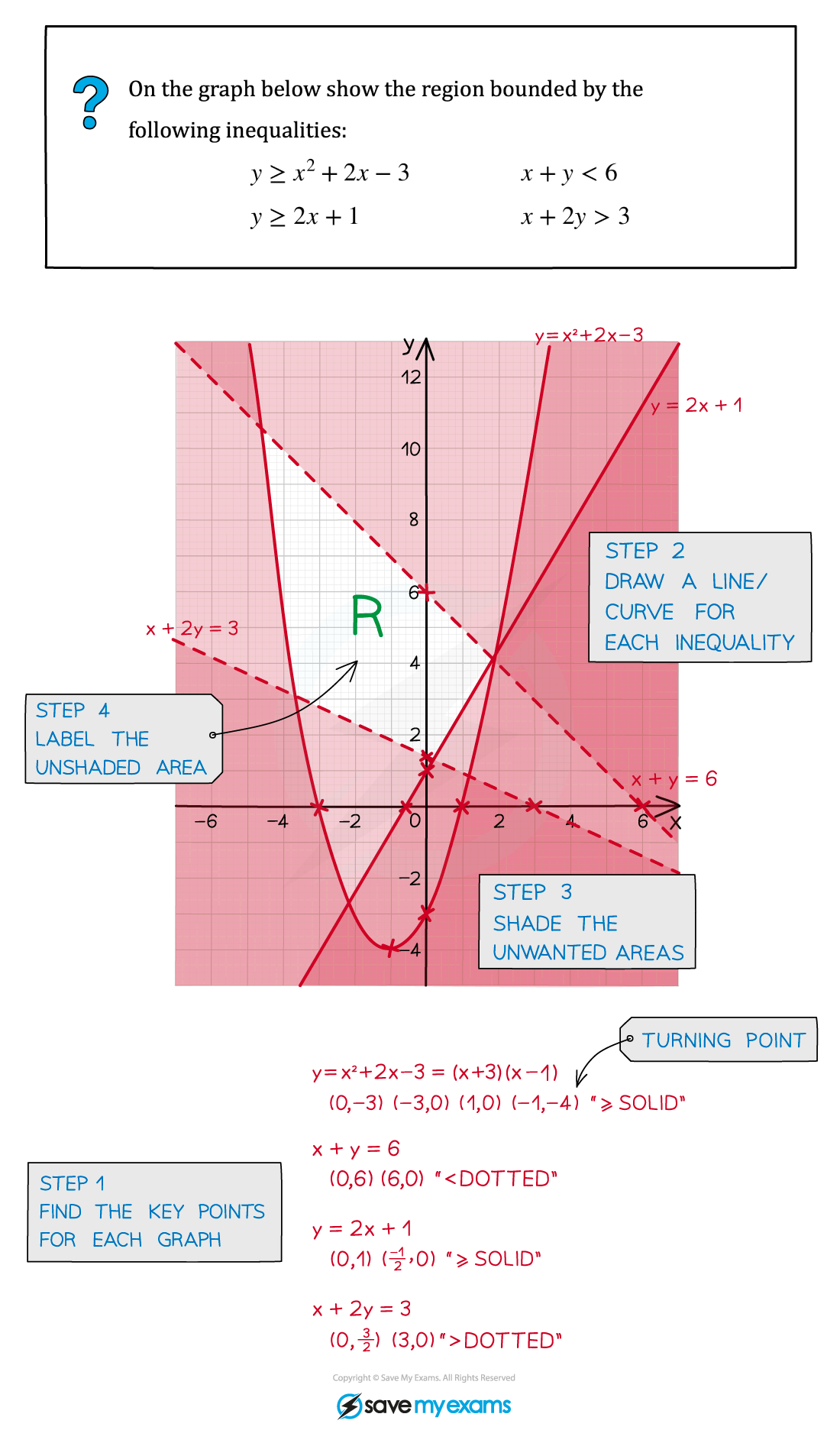
Graphical Representation of Inequalities — This worked example from Save My Exams shows how to find the region R bounded by four inequalities, one of which is quadratic. Notice the use of solid and dotted lines and the shading of unwanted regions. The process is identical to the linear case: draw each boundary and shade the side that doesn't satisfy the inequality.

Solving 1D Quadratic Inequalities using a Graph

A closely related skill is solving an inequality involving only one variable, like $x^{2} + 3 x - 10 < 0$ . You've previously solved quadratic equations; the graphical method is the safest way to solve quadratic inequalities.

Method:

Find the Critical Values: First, solve the corresponding equation to find the roots. For $x^{2} + 3 x - 10 = 0$ , factorising gives $(x + 5) (x - 2) = 0$ , so the roots are $x = - 5$ and $x = 2$ . These are your "critical values".
Sketch the Graph: Draw a quick sketch of the parabola $y = x^{2} + 3 x - 10$ . You know it's a 'U' shape (since the $x^{2}$ term is positive) and it crosses the x-axis at -5 and 2.
Identify the Region:
- If the inequality is < 0, you're looking for where the graph is below the x-axis.
- If the inequality is > 0, you're looking for where the graph is above the x-axis.
Write the Solution:
- For $x^{2} + 3 x - 10 < 0$ , the graph is below the x-axis between the roots. The solution is $- 5 < x < 2$ .
- For $x^{2} + 3 x - 10 > 0$ , the graph is above the x-axis in two separate parts. The solution is $x < - 5$ or $x > 2$ .

This video explains the method clearly.

Solving Quadratic Inequalities - GCSE Higher Maths

This video from 1st Class Maths shows exactly how to use a sketch of a quadratic to solve 1D inequalities. This is a very common source of error if you try to do it without a sketch, so the method is key.

Watch from 00:45 to 04:39. The first part shows how to solve a '< 0' inequality, and the second part shows how to solve a '> 0' inequality. Notice how the solution is written differently in each case.

This image provides a great visual summary of the concept.

Quadratic Inequalities: Graphical Solutions — This image illustrates how the regions on a quadratic graph correspond to the solutions of an inequality. For y < 0, the solution is the x-values where the parabola is below the x-axis. For y > 0, the solution is the x-values where the parabola is above the x-axis.

Part 3: Working Backwards - Finding Inequalities from a Graph

A good test of your understanding is to reverse the problem. You'll be given a graph with a shaded region and asked to write down the inequalities that define it.

Method:

Find the equation of each boundary line (e.g., using gradient-intercept form, $y = m x + c$ ).
Decide on the inequality symbol. Use a test point from within the wanted region (the unshaded part) and substitute it into your equation to figure out if you need <, >, ≤, or ≥.
Check the line type. If the line is dotted, use < or >. If it's solid, use ≤ or ≥.

The first video we watched has an excellent section on this.

Graphical Inequalities & Shaded Regions | GCSE Maths Tutor

Let's revisit the first video to see how to tackle this reverse-style question. This is a great way to consolidate your understanding.

Watch the final example from 22:22 to 27:44. The tutor works backwards from a shaded region to find the three inequalities that define it. Pay close attention to how he determines the inequality sign for each line and remembers to add the 'or equal to' part for the solid lines at the end.

Conclusion

You have now learned a systematic and reliable graphical method for handling inequalities, a topic you previously found challenging. This skill directly builds on your ability to sketch and interpret graphs.

Key Takeaways:

Inequalities define regions, not just lines or points.
The type of line is critical: dotted for < or >, solid for ≤ or ≥.
The test point method is the most reliable way to identify the correct region to shade. For exam purposes, always shade the unwanted region unless told otherwise.
For 1D quadratic inequalities (e.g., $a x^{2} + b x + c > 0$ ), always sketch the parabola to correctly identify the solution set. The solution will either be a single region between the roots or two separate regions outside the roots.

Now, apply the "Error-Loop Method" by working through past-paper questions on this topic. Focus on being precise with your lines and methodical with your shading.

Preview of the Next Lesson:
We have now covered sketching, solving equations, and representing inequalities with graphs. The next lesson, "Apply transformations to the graph of y=f(x): translations, reflections, and stretches", will introduce a new set of skills. You'll learn how to manipulate an entire graph by adjusting its equation, which is a powerful concept in functions.

Recommended resources