Graphical Solutions to Equations

The Fundamental Principle

The core idea is simple but powerful:
If you have two graphs, $y=f(x)$ and $y=g(x)$, the points where they intersect are the points where their $y$-values are identical. Therefore, at any point of intersection, the equation $f(x)=g(x)$ must be true.

The x-coordinates of these intersection points are the solutions to the equation $f(x)=g(x)$.

Let's start by reviewing the basics of this concept.

Scenario 1: Solving f(x) = k (Intersection with a Horizontal Line)

The most straightforward type of question asks you to solve an equation like $f(x)=c$, where $c$ is a constant, using a pre-drawn graph of $y=f(x)$.

This is equivalent to finding the intersection of two graphs:

1. $y=f(x)$ (the curve you are given)
2. $y=c$ (a horizontal line passing through $c$ on the y-axis)

To find the solutions, you simply draw the horizontal line and read the x-coordinates of all intersection points.

This image shows how to solve the equation f(x) = 0.5. A horizontal line is drawn at y = 0.5. The x-coordinates of the points where the line crosses the curve are the solutions. In this case, there are three solutions.

This video from the Ginger Mathematician works through a typical exam question demonstrating this.

Scenario 2: Solving f(x) = g(x) (Intersection of Two Curves)

Sometimes, a question will provide you with two graphs already plotted on the same axes, for example a quadratic and an exponential function. If you are asked to solve the equation $f(x)=g(x)$, the work is already done. You just need to identify the points of intersection and read off their x-coordinates.

Test your understanding!

The image below shows the graph of a function $y=f(x)$.

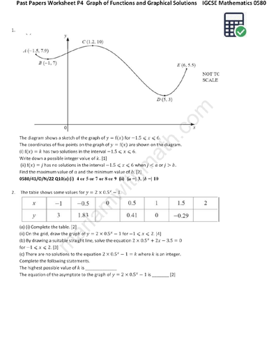
Use the graph in Question 8 to answer the following:
a) Find the solutions to the equation $f(x)=-1$.
b) The equation $f(x)=k$ has only one solution. Write down the value of $k$.

Show answer

a) To solve $f(x)=-1$, you need to draw the horizontal line $y=-1$. This line intersects the curve at three points. Reading off the x-coordinates, the solutions are approximately $x=-1.8$, $x=0$, and $x=1.8$. (Examiners allow a range of answers).

b) For $f(x)=k$ to have only one solution, the horizontal line $y=k$ must touch the curve at only one point. This happens at the local maximum and local minimum points of the graph.

• The local maximum is at $y=1$. So, if $k=1$, there is one solution (a repeated root).
• The local minimum is at $y=-3$. So, if $k=-3$, there is one solution (a repeated root).
  The question is phrased to have a single value, but in this case, there are two possible values for k. Reading the graph, the minimum turning point has a y-value of -3. Let's take $k=-3$. The maximum turning point has a y-value of 1, so $k=1$ is also a valid answer.

Scenario 3: The "Suitable Straight Line" Method

This is the most challenging—and therefore most valuable—type of graphical question. You will be given the graph of a function, say $y=f(x)$, and asked to solve a different equation that looks related but not identical.

Your task is to rearrange the new equation algebraically so that one side becomes $f(x)$. The other side will become the equation of a new line, usually in the form $y=mx+c$.

The Method:

1. Identify the original function, $f(x)$, from the graph you've been given.
2. Take the new equation you need to solve.
3. Manipulate the new equation so that the expression for $f(x)$ appears on one side.
4. The expression on the other side is the "suitable straight line", $y=g(x)$, that you must draw.
5. Draw this new line on the same axes.
6. The x-coordinates of the intersection points between $y=f(x)$ and your new line $y=g(x)$ are the solutions.

This technique is a perfect test of the strategic thinking you want to improve. It combines algebraic manipulation with graphical interpretation.

This video demonstrates this A*-grade skill perfectly.

Let's break down the logic from the video:

• We have the graph of: $y=x^3+3x+4$
• We want to solve: $x^3+5x+2=0$
• Goal: Make the left side of the target equation look like our graph's equation.
  $x^3+5x+2=0$
  We need $x^3+3x+4$. Let's force it to appear.
  $(x^3+3x+4)+2x-2=0$
• Rearrange to the form Graph = Line:
  $x^3+3x+4=-2x+2$
• This tells us the solutions are the x-coordinates of the intersections between the original curve $y=x^3+3x+4$ and the new line $y=-2x+2$.

This is a powerful method that turns a complex problem into a simple case of drawing a straight line.

Conclusion

Today we've transformed your sketching skills from the previous lesson into a powerful tool for solving equations. The key is to understand that intersections are solutions.

Key Takeaways:

• To solve $f(x)=g(x)$, you find the x-coordinates of the intersection points of the graphs $y=f(x)$ and $y=g(x)$.
• Scenario 1 ($f(x)=k$): Draw the horizontal line $y=k$ and find the intersections with the curve $y=f(x)$.
• Scenario 2 (Both graphs given): Simply read the x-coordinates from the existing intersection points.
• Scenario 3 (Disguised equation): This is the crucial skill. Algebraically manipulate the target equation until it is in the form $f(x)=mx+c$, where $y=f(x)$ is the graph you were given. Then, draw the line $y=mx+c$ and find the intersections.

Practice for Mastery:
Now, apply the "Error-Loop Method" by tackling some past paper questions. For the second question in the image LINK (x + 1/x = 4), you would need to use the graph of $y=x+1/x$, draw the line $y=4$, and find the intersections. For more complex problems, remember the algebraic rearrangement step.

Preview of the Next Lesson:
We have learned how to find where two functions are equal by finding their intersection points. In the next lesson, we will extend this idea to find where one function is greater than or less than another. This involves representing and interpreting linear and quadratic inequalities on graphs by identifying solution regions.