Building a Continuous Forward Rate Curve

1. From Discrete to Instantaneous Forward Rates

Let's begin by recalling the concept of forward rates from a no-arbitrage perspective. A forward rate is an interest rate, agreed upon today, for a loan that will be made between two future points in time.

The following video provides a clear derivation of the relationship between spot rates and these discrete forward rates.

The video establishes the relationship using annual compounding. In our work, we use continuous compounding, which simplifies the mathematics. The no-arbitrage principle states that an investment over a period $[0,T_2]$ must yield the same return as an investment over $[0,T_1]$ followed by a reinvestment over $[T_1,T_2]$ at the forward rate $F(T_1,T_2)$.

With continuous compounding, this is expressed as:

where $r(T)$ is the continuously compounded spot rate for maturity $T$.

Taking the natural logarithm of both sides and rearranging for the forward rate gives us:

This is the discrete forward rate over the interval $[T_1,T_2]$.

Our goal, however, is a continuous forward rate curve. This requires us to find the forward rate for an infinitesimally small period in the future. This is known as the instantaneous forward rate, denoted $f(T)$. We find it by taking the limit of our discrete forward rate formula as the interval shrinks to zero, i.e., as $T_2\to T_1$.

2. Deriving the Continuous Forward Rate Curve

Let's formalize the derivation of the instantaneous forward rate. We set $T_1=T$ and $T_2=T+\Delta T$. Our formula for the discrete forward rate becomes:

The instantaneous forward rate $f(T)$ is the limit of this expression as $\Delta T\to 0$:

You'll recognize this as the definition of the derivative for the function $g(T)=r(T)\cdot T$. Therefore:

Applying the product rule for differentiation, we arrive at the fundamental relationship between the instantaneous forward rate and the spot rate curve:

This elegant formula is central to fixed-income mathematics. It shows that the instantaneous forward rate at a given maturity $T$ is the sum of the spot rate at that maturity and the slope of the spot curve at that point, scaled by $T$.

Mathematical and Economic Interpretation

This relationship has direct economic meaning:

• If the spot curve is upward-sloping ($r^{\prime }(T)>0$), then $f(T)>r(T)$. The forward rate is higher than the spot rate, implying the market expects rates to rise.
• If the spot curve is downward-sloping ($r^{\prime }(T)<0$), then $f(T)<r(T)$. The forward rate is lower than the spot rate, implying the market expects rates to fall.
• If the spot curve is flat ($r^{\prime }(T)=0$), then $f(T)=r(T)$. The forward rate equals the spot rate.

The following discussion provides a more detailed look at the instantaneous forward rate, including an alternative derivation from the price of a zero-coupon bond.

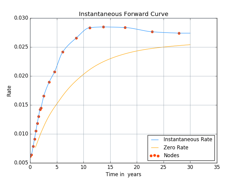
The chart below visualizes this relationship. Where the spot ("Zero Rate") curve is rising, the instantaneous forward curve lies above it. Where the spot curve begins to flatten, the two curves converge.

3. Python Implementation

Now, let's implement this derivation in Python. We will extend the YieldCurve class from the previous lesson. The choice of scipy.interpolate.CubicSpline was deliberate; not only does it provide a smooth curve, but its derivatives can be computed analytically. This makes calculating the forward curve remarkably straightforward.

The CubicSpline object has a .derivative(nu=k) method, which returns a new spline object representing the $k$-th derivative of the original. We need the first derivative ($k=1$).

Here is the updated YieldCurve class. We will add two new methods: forward_rate to compute the rate at a single point, and plot_all_curves to visualize the spot and forward curves together.

import numpy as np
import matplotlib.pyplot as plt
from scipy.interpolate import CubicSpline
from scipy.optimize import brentq
from typing import List, Dict, Tuple




# ========== CLASS 1: THE UPDATED YIELD CURVE OBJECT ==========
class YieldCurve:
    """
    Represents a continuous yield curve and allows derivation of the forward curve.
    """
    def __init__(self, tenors: List[float], rates: List[float]):
        self._spline = CubicSpline(tenors, rates, bc_type='natural')
        self._spline_deriv = self._spline.derivative(nu=1)
        self.tenors = np.array(tenors)
        self.rates = np.array(rates)

    def spot_rate(self, t: float) -> float:
        """Returns the continuously compounded spot rate for a given tenor."""
        return self._spline(t)

    def forward_rate(self, t: float) -> float:
        """Returns the continuously compounded instantaneous forward rate for a given tenor."""
        if t == 0:



            # At t=0, r(0)=f(0). The derivative term t*r'(t) is zero.
            return self.spot_rate(0)
            
        r_t = self.spot_rate(t)
        r_prime_t = self._spline_deriv(t)
        



        # The core formula: f(t) = r(t) + t * r'(t)
        return r_t + t * r_prime_t

    def plot_all_curves(self, t_max: float = None):
        """Plots the discrete points and the continuous spot and forward curves."""
        if t_max is None:
            t_max = self.tenors.max()
        
        plot_tenors = np.linspace(0, t_max, 300)
        spot_rates = self.spot_rate(plot_tenors)



        # Vectorize the forward_rate calculation for plotting
        forward_rates = np.array([self.forward_rate(t) for t in plot_tenors])
        
        plt.figure(figsize=(12, 7))
        plt.plot(self.tenors, self.rates, 'o', markersize=8, label='Bootstrapped Points')
        plt.plot(plot_tenors, spot_rates, '-', lw=2, label='Spot Curve')
        plt.plot(plot_tenors, forward_rates, '--', lw=2, label='Forward Curve')
        
        plt.title('Spot and Forward Rate Curves')
        plt.xlabel('Tenor (Years)')
        plt.ylabel('Continuously Compounded Rate')
        plt.grid(True, linestyle='--', alpha=0.6)
        plt.legend()
        plt.show()




# (The BondBootstrapper and CurveFactory classes from the previous lesson remain unchanged)
# ========== CLASS 2: THE BOOTSTRAPPING ENGINE ==========
class BondBootstrapper:
    def bootstrap(self, bonds: List[Dict]) -> Tuple[np.ndarray, np.ndarray]:
        bonds_sorted = sorted(bonds, key=lambda b: b['maturity'])
        known_tenors = [0.0]
        known_rates = [0.0] 
        for bond in bonds_sorted:
            rate = brentq(
                lambda r: self._price_bond(bond, r, known_tenors, known_rates) - bond['price'],
                a=-0.05, b=0.50
            )
            known_tenors.append(bond['maturity'])
            known_rates.append(rate)
        return np.array(known_tenors), np.array(known_rates)

    def _price_bond(self, bond: Dict, final_rate: float, known_tenors: List, known_rates: List) -> float:
        maturity, coupon_rate, frequency, face_value = bond['maturity'], bond['coupon'], bond['frequency'], bond.get('face_value', 100.0)
        coupon_payment = face_value * coupon_rate / frequency
        num_periods = int(round(maturity * frequency))
        price = 0.0
        for i in range(1, num_periods + 1):
            t = i / frequency
            cash_flow = coupon_payment
            if i == num_periods:
                cash_flow += face_value
            if t < maturity:
                rate_t = np.interp(t, known_tenors, known_rates)
            else:
                rate_t = final_rate
            price += cash_flow * np.exp(-rate_t * t)
        return price




# ========== CLASS 3: THE FACTORY INTERFACE ==========
class CurveFactory:
    @staticmethod
    def create_from_bonds(bonds: List[Dict]) -> YieldCurve:
        bootstrapper = BondBootstrapper()
        tenors, rates = bootstrapper.bootstrap(bonds)
        return YieldCurve(list(tenors), list(rates))




# ========== RUN THE WORKFLOW ==========




# 1. Define the same market data from the previous lesson
market_bonds = [
    {'maturity': 1.0, 'coupon': 0.050, 'price': 100.0, 'frequency': 2},
    {'maturity': 2.0, 'coupon': 0.055, 'price': 100.0, 'frequency': 2},
    {'maturity': 3.0, 'coupon': 0.058, 'price': 100.0, 'frequency': 2},
    {'maturity': 5.0, 'coupon': 0.062, 'price': 100.0, 'frequency': 2},
    {'maturity': 7.0, 'coupon': 0.065, 'price': 100.0, 'frequency': 2},
    {'maturity': 10.0, 'coupon': 0.068, 'price': 100.0, 'frequency': 2},
    {'maturity': 30.0, 'coupon': 0.070, 'price': 100.0, 'frequency': 2},
]




# 2. Use the factory to construct the curve
full_curve = CurveFactory.create_from_bonds(market_bonds)




# 3. Use the new plotting method to visualize both curves
full_curve.plot_all_curves()




# 4. Calculate and print a specific forward rate
t_forward = 5.0
f_rate = full_curve.forward_rate(t_forward)
s_rate = full_curve.spot_rate(t_forward)
print(f"At {t_forward} years:")
print(f"  Spot Rate    = {s_rate:.4%}")
print(f"  Forward Rate = {f_rate:.4%}")

Code Analysis

• In the YieldCurve.__init__, we now pre-calculate and store the spline's first derivative (self._spline_deriv). This is efficient as it's done only once.
• The forward_rate method is a direct translation of our formula $f(T)=r(T)+T\cdot r^{\prime }(T)$. It calls the spline and its derivative to get the necessary values.
• The plot_all_curves method generates a smooth plot by evaluating both spot_rate and forward_rate across a dense range of tenors. The resulting graph clearly shows the relationship between the two curves, confirming our theoretical understanding.

The QuantLib-Python companion article (LINK) further illustrates this concept in a professional library setting. The multiple calls to curve.forwardRate(...) in that code are analogous to the method we just built, demonstrating that this is a standard and essential feature of any yield curve object.

Conclusion

In this lesson, you have successfully derived the continuous forward rate curve from the spot rate curve you built previously. This involved both a rigorous mathematical derivation and a practical Python implementation.

Key Takeaways:

• The instantaneous forward rate $f(T)$ is the theoretical rate for an infinitesimal loan at a future time $T$.
• It is mathematically linked to the spot rate curve $r(T)$ by the formula: $f(T)=r(T)+T\cdot r^{\prime }(T)$.
• This relationship means the forward curve will lie above an upward-sloping spot curve and below a downward-sloping one.
• Using a CubicSpline to model the spot curve allows for straightforward calculation of its derivative, making the implementation of the forward curve efficient and elegant.

You have now constructed two of the three most important interest rate curves. In the next lesson, we will complete the trio by deriving the par-yield curve from the spot curve, providing you with a complete set of tools for analyzing the term structure of interest rates.