Introduction
In our recent lessons, we have progressively built a sophisticated toolkit for analyzing the term structure of interest rates. Starting with raw bond data, you learned to bootstrap a discrete spot curve, fit a continuous CubicSpline to it, and then derive the continuous instantaneous forward rate curve. You now have a Python YieldCurve class that can provide both the spot rate and forward rate for any maturity .
This lesson will complete the trio of fundamental interest rate curves by focusing on the par-yield curve. We will define what a par yield represents, derive its mathematical relationship to the spot rate curve you've already constructed, and explain its significant practical role in financial markets. By the end of this lesson, you will have implemented the logic to compute and visualize all three curves—spot, forward, and par—from a single underlying model.
1. What is a Par-Yield Curve?
Before we dive into the math, let's establish the core concept.
A par bond is a bond whose market price is exactly equal to its face value (typically 100).
The par yield for a specific maturity is the coupon rate that a hypothetical bond of that maturity must have in order to be priced at par.
A par-yield curve is a plot of these par yields against their corresponding maturities.
Essentially, for each point on the curve, you are asking: "What coupon rate would make a new bond with maturity trade at exactly 100, given today's term structure of interest rates?"
The comment by user closedloop in the following Stack Overflow thread provides a succinct and practical definition.
How do I construct a treasury yield curve in QuantLib? - Comment
This is a very short reading. Focus on the comment exchange in the middle of the page.
Read the comment from user closedloop which starts "the treasury curves are par rates...". This captures the essential definition of a par rate in contrast to a zero rate (spot rate).
In practice, the most recently issued government bonds (called "on-the-run" treasuries) trade at prices very close to par. Their coupon rates are set based on prevailing market conditions at the time of issuance. As a result, a collection of on-the-run treasuries of different maturities effectively forms a par-yield curve. This is why par curves are often what is directly observed and quoted in the market.
The image below shows a table of such "par Treasuries," where the coupon rate (listed as "Yield") for each tenor has been set so that the price is exactly 100.

2. Deriving the Par Yield from the Spot Curve
Now that we have the concept, we can formalize the derivation. Our goal is to find the par yield for a given maturity , denoted , using our existing continuous spot rate curve .
Let's consider a bond with:
- Face Value:
- Maturity: years
- Coupon Payment Frequency: times per year
- Coupon Rate:
The coupon payment per period is . The payment times are for , where is the total number of payments.
From our previous work, the price of this bond, discounted using the continuous spot rate curve , is:
We can separate the coupon and principal payments:
By definition, for a par bond, , and the coupon rate is the par yield, . Substituting these in, we get:
We can now solve for . First, divide the entire equation by :
Rearranging to isolate the term with :
Finally, solving for the par yield :
This is the key formula. It directly expresses the par yield for maturity as a function of the entire spot rate curve up to that maturity. The term is the price of a zero-coupon bond maturing at , and the summation in the denominator is the present value of an annuity of $1 per period, with each payment discounted by its corresponding spot rate.
The following paper provides a similar derivation using discrete compounding, but the underlying principle of setting the price to par and solving for the coupon is identical.
The Arithmetics of Par, Spot and Forward Curves
This paper by Levan Gvilava provides a rigorous mathematical treatment of the relationships between different yield curves.
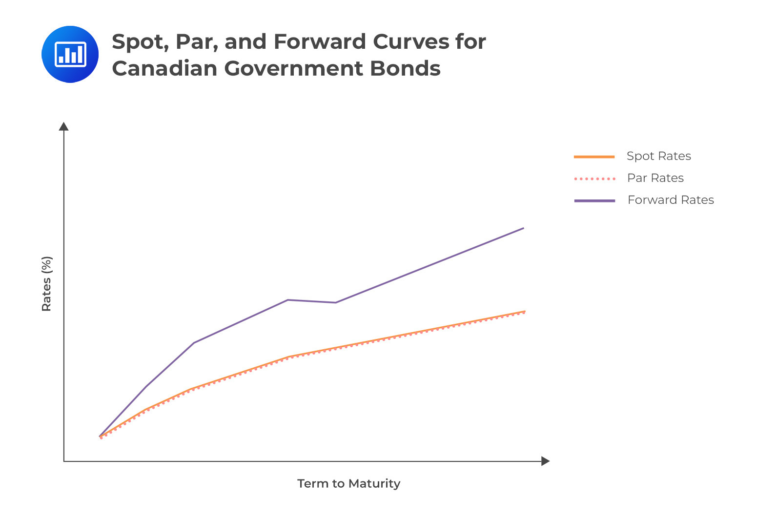
Focus on section 3.3, "The Ordering of Par and Spot Curves." Equation (12) is the discrete-compounding equivalent of our starting point. The author then discusses the mathematical relationship between the shapes of the spot and par curves. Note the conclusions (points 8 and 9): if the spot curve is upward-sloping, it lies above the par curve. If it's downward-sloping, the par curve lies above the spot curve.
The reasoning behind this relationship is that the par yield is a coupon-weighted average of the spot rates. For an upward-sloping curve, the earlier, lower spot rates drag the par yield down below the final spot rate . Conversely, for a downward-sloping curve, the earlier, higher spot rates pull the par yield up.
This chart visually summarizes the typical relationship in a normal, upward-sloping yield curve environment.
3. Python Implementation
Let's integrate this new capability into our YieldCurve class. We will add a par_yield method that implements our derived formula and update the plotting method to visualize all three curves.
import numpy as np
import matplotlib.pyplot as plt
from scipy.interpolate import CubicSpline
from scipy.optimize import brentq
from typing import List, Dict, Tuple


# ========== CLASS 1: THE YIELD CURVE OBJECT (UPDATED) ==========
class YieldCurve:
    """
    Represents a continuous yield curve and allows derivation of forward and par curves.
    """
    def __init__(self, tenors: List[float], rates: List[float]):
        self._spline = CubicSpline(tenors, rates, bc_type='natural')
        self._spline_deriv = self._spline.derivative(nu=1)
        self.tenors = np.array(tenors)
        self.rates = np.array(rates)

    def spot_rate(self, t: float) -> float:
        """Returns the continuously compounded spot rate for a given tenor."""
        return self._spline(t)

    def forward_rate(self, t: float) -> float:
        """Returns the continuously compounded instantaneous forward rate for a given tenor."""
        if t == 0:
            return self.spot_rate(0)
        r_t = self.spot_rate(t)
        r_prime_t = self._spline_deriv(t)
        return r_t + t * r_prime_t

    def par_yield(self, t: float, frequency: int = 2) -> float:
        """
        Calculates the par yield for a given maturity t.
        Assumes semi-annual coupons by default.
        """
        if t == 0:
            return self.spot_rate(0)

        num_periods = int(round(t * frequency))
        payment_times = np.linspace(1/frequency, t, num_periods)


        # Calculate the price of a zero-coupon bond maturing at T
        # This is the numerator term: 1 - e^(-r(T)T)
        zero_price = np.exp(-self.spot_rate(t) * t)


        # Calculate the annuity factor (the summation in the denominator)
        # Sum of discount factors for each coupon payment
        annuity_factor = 0.0
        for t_i in payment_times:
            annuity_factor += np.exp(-self.spot_rate(t_i) * t_i)


        # Par Yield Formula: y_p = m * (1 - P(0,T)) / (Annuity Factor)
        # Note: the annuity factor as calculated is sum(e^-rt), our formula has sum(1/m * e^-rt)
        # So we use m / (sum(e^-rt)) which is equivalent to 1 / (1/m * sum(e^-rt))
        par_yield = frequency * (1 - zero_price) / annuity_factor

        return par_yield

    def plot_all_curves(self, t_max: float = None, frequency: int = 2):
        """Plots the discrete points and the continuous spot, forward, and par curves."""
        if t_max is None:
            t_max = self.tenors.max()

        plot_tenors = np.linspace(0.1, t_max, 300) # Start from 0.1 to avoid t=0 issues in plotting
        spot_rates = self.spot_rate(plot_tenors)
        forward_rates = np.array([self.forward_rate(t) for t in plot_tenors])
        par_yields = np.array([self.par_yield(t, frequency) for t in plot_tenors])

        plt.figure(figsize=(14, 8))
        plt.plot(self.tenors, self.rates, 'o', markersize=8, label='Bootstrapped Points')
        plt.plot(plot_tenors, spot_rates, '-', lw=2, label='Spot Curve')
        plt.plot(plot_tenors, forward_rates, '--', lw=2, label='Forward Curve')
        plt.plot(plot_tenors, par_yields, ':', lw=2, label=f'Par Curve ({frequency} p.a.)')

        plt.title('Spot, Forward, and Par-Yield Curves')
        plt.xlabel('Tenor (Years)')
        plt.ylabel('Continuously Compounded Rate / Par Yield')
        plt.grid(True, linestyle='--', alpha=0.6)
        plt.legend()
        plt.show()


```grasp
{
  "type": "exercise",
  "id": "0510b6fa-c37d-40fd-a80a-76052bc2de46"
}
(The BondBootstrapper and CurveFactory classes from the previous lessons remain unchanged)
========== CLASS 2: THE BOOTSTRAPPING ENGINE ==========
class BondBootstrapper:
# ... (code from previous lesson)
def bootstrap(self, bonds: List[Dict]) -> Tuple[np.ndarray, np.ndarray]:
    bonds_sorted = sorted(bonds, key=lambda b: b['maturity'])
    known_tenors = [0.0]
    known_rates = [0.0]
    for bond in bonds_sorted:
        rate = brentq(
            lambda r: self._price_bond(bond, r, known_tenors, known_rates) - bond['price'],
            a=-0.05, b=0.50
        )
        known_tenors.append(bond['maturity'])
        known_rates.append(rate)


    # Ensure rates at tenor 0 is based on interpolation rather than a fixed 0.
    # This is a small refinement for better behavior at the short end.
    if len(known_tenors) > 2:
        f = CubicSpline(known_tenors[1:], known_rates[1:], bc_type='natural')
        known_rates[0] = f(0) if f(0) > 0 else 0.0

    return np.array(known_tenors), np.array(known_rates)

def _price_bond(self, bond: Dict, final_rate: float, known_tenors: List, known_rates: List) -> float:
    maturity, coupon_rate, frequency, face_value = bond['maturity'], bond['coupon'], bond['frequency'], bond.get('face_value', 100.0)
    coupon_payment = face_value * coupon_rate / frequency
    num_periods = int(round(maturity * frequency))
    price = 0.0

    temp_spline = CubicSpline(known_tenors + [maturity], known_rates + [final_rate], bc_type='natural')

    for i in range(1, num_periods + 1):
        t = i / frequency
        cash_flow = coupon_payment
        if i == num_periods:
            cash_flow += face_value

        rate_t = temp_spline(t)
        price += cash_flow * np.exp(-rate_t * t)
    return price
========== CLASS 3: THE FACTORY INTERFACE ==========
class CurveFactory:
@staticmethod
def create_from_bonds(bonds: List[Dict]) -> YieldCurve:
bootstrapper = BondBootstrapper()
tenors, rates = bootstrapper.bootstrap(bonds)
return YieldCurve(list(tenors), list(rates))
========== RUN THE WORKFLOW ==========
1. Define market data (using par bonds for simplicity, as in previous lesson)
market_bonds = [
{'maturity': 1.0, 'coupon': 0.050, 'price': 100.0, 'frequency': 2},
{'maturity': 2.0, 'coupon': 0.055, 'price': 100.0, 'frequency': 2},
{'maturity': 3.0, 'coupon': 0.058, 'price': 100.0, 'frequency': 2},
{'maturity': 5.0, 'coupon': 0.062, 'price': 100.0, 'frequency': 2},
{'maturity': 7.0, 'coupon': 0.065, 'price': 100.0, 'frequency': 2},
{'maturity': 10.0, 'coupon': 0.068, 'price': 100.0, 'frequency': 2},
{'maturity': 30.0, 'coupon': 0.070, 'price': 100.0, 'frequency': 2},
]
2. Use the factory to construct the curve object
full_curve = CurveFactory.create_from_bonds(market_bonds)
3. Use the updated plotting method to visualize all three curves
full_curve.plot_all_curves(t_max=30.0)
```grasp
{
  "type": "exercise",
  "id": "a7d8d9e5-77bc-40e8-9249-3d1d80a00962"
}
Code Analysis
par_yieldmethod: This is a direct implementation of our derived formula. It loops through the payment dates up to maturityt, calculates the present value of each $1 coupon using thespot_ratemethod, sums them up to get the annuity factor, and applies the final formula.plot_all_curvesmethod: This is now enhanced to calculate and plot the par-yield curve alongside the spot and forward curves, providing a comprehensive visualization of the term structure.- Refinement in
BondBootstrapper: I've added a small refinement to the bootstrapping logic. Instead of fixing the rate at t=0 to 0.0, it now back-extrapolates from the fitted curve. This can lead to a more stable curve at the very short end, though for most applications the difference is minor. The change in_price_bondto use a temporary spline for each root-finding step also makes the bootstrapping more robust.
The resulting plot clearly demonstrates the relationships we discussed: the forward curve lies above the spot curve, which in turn lies above the par curve, exactly as expected for this upward-sloping data.
Conclusion
In this lesson, you have rounded out your understanding of the fundamental interest rate curves by deriving and implementing the par-yield curve.
Key Takeaways:
- A par-yield curve shows the coupon rate that a bond of a given maturity must have to trade at par.
- Par curves are practically important as they often represent what is directly quoted in the market (e.g., from on-the-run Treasury bonds).
- The par yield can be derived directly from the spot rate curve using the formula:
- For an upward-sloping term structure, the curves are typically ordered from top to bottom: Forward > Spot > Par. The reverse is true for a downward-sloping (inverted) curve.
You now possess a complete theoretical and practical framework for constructing, interpreting, and visualizing the spot, forward, and par-yield curves. This is the bedrock of modern fixed-income analysis.
In our next lesson, we will begin to apply this powerful framework to price more complex securities. We will start by modeling and pricing Floating Rate Notes (FRNs), whose cash flows are not fixed but are instead linked to future interest rates—a concept directly connected to the forward curve you have just mastered.