Yield Curve Analysis: YTM, Spot, and Forward

1. The "YTM Curve" and its Primary Flaw: The Coupon Effect

You'll often hear practitioners talk about the "yield curve" by simply referring to a plot of the Yields-to-Maturity (YTMs) of government bonds with different maturities. While intuitive, this approach has a significant theoretical flaw known as the coupon effect.

Recall that YTM is the single constant interest rate that discounts all of a bond's cash flows to match its market price. The problem is that this single rate is a complex weighted average of the true spot rates that should be used for each cash flow. The weights in this average are the cash flows themselves. Therefore, two bonds with the same maturity but different coupon rates will have different cash flow streams, leading to different YTMs—even if they exist in the exact same interest rate environment (i.e., priced off the same spot curve).

The video below from Bionic Turtle provides an excellent spreadsheet-based demonstration of this coupon effect.

As the video demonstrates, the YTM of a bond is "contaminated" by its own coupon rate. A higher coupon bond gives more weight to the earlier, lower spot rates (in a normal upward-sloping curve), pulling its YTM down relative to a lower coupon bond of the same maturity. This inconsistency is why, for precise valuation and risk management, we derive and use a single, unified spot curve, from which all other consistent curves (par, forward) can be generated.

2. The Mathematical Ordering of Curves

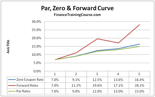
Having established why the YTM curve is flawed, let's focus on the theoretically consistent curves: spot, forward, and par. In the previous lesson, we saw that for an upward-sloping curve, they tend to be ordered: Forward > Spot > Par. Now, let's look at the mathematical basis for this relationship.

The paper "The Arithmetics of Par, Spot and Forward Curves" provides concise derivations for these orderings.

From these derivations, we can summarize the strict ordering of the curves based on the shape of the spot curve:

• Upward-Sloping (Normal) Spot Curve: Forward Curve > Spot Curve > Par Curve
• Downward-Sloping (Inverted) Spot Curve: Par Curve > Spot Curve > Forward Curve
• Flat Spot Curve: Forward Curve = Spot Curve = Par Curve

The YTMs of individual bonds will generally lie around the par curve but will not form a smooth line, instead scattering based on their specific coupon rates.

This diagram clearly visualizes the relationship for a typical upward-sloping curve.

3. Visualizing the Curves in Python

Now, let's bring all these concepts together in our Python code. We will calculate the YTM for each of our input bonds and then create a comprehensive plot that visualizes all four curves—spot, forward, par, and the individual YTMs.

First, we need a function to calculate the YTM for a single bond. This involves finding the root of the price-yield relationship, which is a familiar task.

# Helper function to calculate price with a single rate (YTM)
def _price_with_single_rate(bond: Dict, ytm: float) -> float:
    maturity, coupon_rate, frequency = bond['maturity'], bond['coupon'], bond['frequency']
    face_value = bond.get('face_value', 100.0)
    
    coupon_payment = face_value * coupon_rate / frequency
    num_periods = int(round(maturity * frequency))
    price = 0.0

    for i in range(1, num_periods + 1):
        cash_flow = coupon_payment
        if i == num_periods:
            cash_flow += face_value
        



        # All cash flows discounted at the same rate 'ytm'
        # Using continuous compounding to match our curve framework
        price += cash_flow * np.exp(-ytm * (i / frequency))
        
    return price




# YTM calculation function using a root-finder
def calculate_ytm(bond: Dict) -> float:
    """Calculates the continuously compounded YTM for a given bond."""
    try:
        ytm = brentq(
            lambda y: _price_with_single_rate(bond, y) - bond['price'],
            a=-0.05, b=0.50 # Search range for YTM
        )
        return ytm
    except ValueError:
        return np.nan # Return NaN if root not found

Next, we update the plot_all_curves method in our YieldCurve class to include the YTMs. Note that we will plot YTMs as distinct points ('x') to emphasize that they don't form a single, theoretically consistent curve.

Here is the complete, updated code block.

import numpy as np
import matplotlib.pyplot as plt
from scipy.interpolate import CubicSpline
from scipy.optimize import brentq
from typing import List, Dict, Tuple




# ========== HELPER FUNCTIONS FOR YTM ==========
def _price_with_single_rate(bond: Dict, ytm: float) -> float:
    """Calculates bond price using a single continuously compounded rate (ytm)."""
    maturity, coupon_rate, frequency = bond['maturity'], bond['coupon'], bond['frequency']
    face_value = bond.get('face_value', 100.0)
    
    coupon_payment = face_value * coupon_rate / frequency
    num_periods = int(round(maturity * frequency))
    price = 0.0

    for i in range(1, num_periods + 1):
        cash_flow = coupon_payment
        if i == num_periods:
            cash_flow += face_value
        price += cash_flow * np.exp(-ytm * (i / frequency))
    return price

def calculate_ytm(bond: Dict) -> float:
    """Calculates the continuously compounded YTM for a given bond."""
    try:
        return brentq(lambda y: _price_with_single_rate(bond, y) - bond['price'], a=-0.05, b=0.5)
    except (ValueError, RuntimeError):
        return np.nan




# ========== CLASS 1: THE YIELD CURVE OBJECT (UPDATED PLOTTING) ==========
class YieldCurve:
    """
    Represents a continuous yield curve and allows derivation of forward and par curves.
    """
    def __init__(self, tenors: List[float], rates: List[float]):
        self._spline = CubicSpline(tenors, rates, bc_type='natural')
        self._spline_deriv = self._spline.derivative(nu=1)
        self.tenors = np.array(tenors)
        self.rates = np.array(rates)

    def spot_rate(self, t: float) -> float:
        return self._spline(t)

    def forward_rate(self, t: float) -> float:
        if t == 0: return self.spot_rate(0)
        r_t, r_prime_t = self.spot_rate(t), self._spline_deriv(t)
        return r_t + t * r_prime_t
        
    def par_yield(self, t: float, frequency: int = 2) -> float:
        if t == 0: return self.spot_rate(0)
        num_periods = int(round(t * frequency))
        payment_times = np.linspace(1/frequency, t, num_periods)
        zero_price = np.exp(-self.spot_rate(t) * t)
        annuity_factor = sum(np.exp(-self.spot_rate(ti) * ti) for ti in payment_times)
        return frequency * (1 - zero_price) / annuity_factor

    def plot_all_curves(self, input_bonds: List[Dict], t_max: float = None, frequency: int = 2):
        """
        Plots spot, forward, par curves, and the YTMs of the input bonds.
        """
        if t_max is None:
            t_max = self.tenors.max()
        



        # Calculate YTMs for the input bonds
        bond_maturities = [b['maturity'] for b in input_bonds]
        bond_ytms = [calculate_ytm(b) for b in input_bonds]
        
        plot_tenors = np.linspace(0.1, t_max, 300)
        spot_rates = self.spot_rate(plot_tenors)
        forward_rates = np.array([self.forward_rate(t) for t in plot_tenors])
        par_yields = np.array([self.par_yield(t, frequency) for t in plot_tenors])
        
        plt.figure(figsize=(14, 8))



        # Plot the curves
        plt.plot(plot_tenors, spot_rates, '-', lw=2, label='Spot Curve (ZCYC)', color='blue')
        plt.plot(plot_tenors, forward_rates, '--', lw=2, label='Forward Curve', color='green')
        plt.plot(plot_tenors, par_yields, ':', lw=2, label=f'Par Curve ({frequency} p.a.)', color='red')
        



        # Plot the individual bond data
        plt.plot(self.tenors, self.rates, 'o', markersize=8, label='Bootstrapped Spot Rates', color='blue')
        plt.plot(bond_maturities, bond_ytms, 'x', markersize=10, mew=2, label='Bond YTMs', color='purple')
        
        plt.title('Comparison of YTM, Spot, Forward, and Par-Yield Curves')
        plt.xlabel('Tenor (Years)')
        plt.ylabel('Rate')
        plt.grid(True, linestyle='--', alpha=0.6)
        plt.legend()
        plt.show()




# (The BondBootstrapper and CurveFactory classes remain unchanged from the previous lesson)
# ========== CLASS 2: THE BOOTSTRAPPING ENGINE ==========
class BondBootstrapper:
    def bootstrap(self, bonds: List[Dict]) -> Tuple[np.ndarray, np.ndarray]:
        bonds_sorted = sorted(bonds, key=lambda b: b['maturity'])
        known_tenors, known_rates = [0.0], [0.0]
        for bond in bonds_sorted:
            rate = brentq(lambda r: self._price_bond(bond, r, known_tenors, known_rates) - bond['price'], a=-0.05, b=0.5)
            known_tenors.append(bond['maturity'])
            known_rates.append(rate)
        if len(known_tenors) > 2:
            f = CubicSpline(known_tenors[1:], known_rates[1:], bc_type='natural')
            known_rates[0] = float(f(0)) if float(f(0)) > 0 else 0.0
        return np.array(known_tenors), np.array(known_rates)

    def _price_bond(self, bond: Dict, final_rate: float, known_tenors: List, known_rates: List) -> float:
        maturity, coupon_rate, frequency = bond['maturity'], bond['coupon'], bond['frequency']
        face_value = bond.get('face_value', 100.0)
        coupon_payment = face_value * coupon_rate / frequency
        num_periods = int(round(maturity * frequency))
        price = 0.0
        temp_spline = CubicSpline(known_tenors + [maturity], known_rates + [final_rate], bc_type='natural')
        for i in range(1, num_periods + 1):
            t = i / frequency
            cash_flow = coupon_payment + face_value if i == num_periods else coupon_payment
            price += cash_flow * np.exp(-temp_spline(t) * t)
        return price




# ========== CLASS 3: THE FACTORY INTERFACE ==========
class CurveFactory:
    @staticmethod
    def create_from_bonds(bonds: List[Dict]) -> YieldCurve:
        bootstrapper = BondBootstrapper()
        tenors, rates = bootstrapper.bootstrap(bonds)
        return YieldCurve(list(tenors), list(rates))




# ========== RUN THE WORKFLOW ==========
# 1. Define market data with varying coupons to illustrate the coupon effect
market_bonds_varied_coupons = [
    {'maturity': 1.0, 'coupon': 0.02, 'price': 99.50, 'frequency': 2},
    {'maturity': 2.0, 'coupon': 0.055, 'price': 102.3, 'frequency': 2}, # High coupon -> premium price
    {'maturity': 3.0, 'coupon': 0.03, 'price': 97.0, 'frequency': 2}, # Low coupon -> discount price
    {'maturity': 5.0, 'coupon': 0.062, 'price': 104.0, 'frequency': 2},
    {'maturity': 7.0, 'coupon': 0.035, 'price': 92.5, 'frequency': 2},
    {'maturity': 10.0, 'coupon': 0.04, 'price': 91.0, 'frequency': 2},
    {'maturity': 30.0, 'coupon': 0.045, 'price': 85.0, 'frequency': 2},
]




# 2. Use the factory to construct the curve object
full_curve = CurveFactory.create_from_bonds(market_bonds_varied_coupons)




# 3. Use the updated plotting method to visualize everything
full_curve.plot_all_curves(input_bonds=market_bonds_varied_coupons, t_max=30.0)

The resulting plot is the central takeaway of this lesson. You can clearly see the smooth, theoretically related Spot, Forward, and Par curves. Their ordering (Forward > Spot > Par) matches the theory for an upward-sloping curve. In contrast, the Bond YTMs (purple 'x' markers) do not lie on a single smooth curve. They are scattered, demonstrating the coupon effect in action. This visualization makes it evident why we bootstrap a spot curve rather than simply connecting the dots between YTMs.

Conclusion

In this lesson, we synthesized our knowledge of the term structure by visualizing and contrasting the four main types of yield curves derived from a single set of market data.

Key Takeaways:

• YTM is Bond-Specific: The Yield-to-Maturity is influenced by a bond's specific coupon rate (the "coupon effect"). A plot of YTMs from different bonds does not form a theoretically consistent term structure.
• Theoretically Consistent Curves: The spot, forward, and par curves are all consistent representations of the term structure of interest rates. The spot curve (or ZCYC) is the most fundamental.
• Mathematical Ordering: For a normal, upward-sloping yield curve, the ordering is Forward > Spot > Par. This relationship inverts for a downward-sloping curve, and all three are identical for a flat curve.
• The Spot Curve as the Foundation: The ultimate goal of bootstrapping is to extract the one true underlying spot curve. From it, we can price any bond or derivative consistently, and derive other useful representations like the forward and par curves.

You are now equipped with a comprehensive understanding of how these critical curves relate to one another, both mathematically and practically.

In our next lesson, we will delve into the economic interpretation of yield curve shapes. We'll explore what normal, inverted, flat, and humped yield curves signal about the state of the economy and market expectations for future growth, inflation, and central bank policy.