Introduction
Welcome to the final lesson of this module. In our previous lessons, we explored linear, polynomial, and cubic spline interpolation individually, culminating in a practical Python implementation of cubic splines. You now have the building blocks for constructing a continuous yield curve. The crucial question remains: which block is the right one for the job, and why?
Today, we will answer that question by directly comparing these three methods. Our goal is to apply them to the same set of bootstrapped spot rates and critically analyze the resulting spot and, more importantly, forward rate curves. This comparative analysis will visually and mathematically demonstrate the strengths and weaknesses of each approach, solidifying why cubic splines are the preferred method in financial engineering for balancing smoothness and stability.
1. The Importance of Smoothness
Before we dive into the comparison, let's revisit why the smoothness of an interpolated curve is so critical. The primary reason is its impact on the forward rate curve. Recall the relationship between the instantaneous forward rate and the continuously compounded spot rate :
This equation shows that the forward rate depends on the spot rate's first derivative, . A "smooth" interpolator is one that has continuous derivatives.
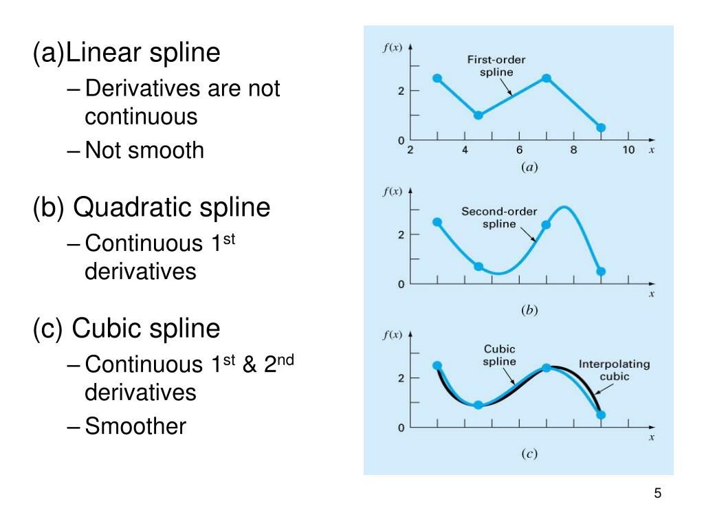
As you can see, if our spot curve is not continuously differentiable (like a linear spline), our forward curve will have jumps or discontinuities. Such jumps are economically implausible, as they would imply predictable, instantaneous arbitrage opportunities. Therefore, our evaluation of interpolation methods will heavily focus on the quality of the forward curve they produce.
2. Setting Up the Comparison in Python
To perform a fair comparison, we will use a single, challenging dataset of bootstrapped spot rates and apply each of our three interpolation methods to it. We will then plot the resulting spot curves and their corresponding forward curves on the same axes.
The dataset we'll use is taken from the paper "An investigation into popular methods for constructing yield curves" and is designed to expose the flaws in naive interpolation methods.
Here is the complete Python script we will use. Let's walk through it step-by-step.
import numpy as np
import matplotlib.pyplot as plt
from scipy.interpolate import interp1d, CubicSpline, BarycentricInterpolator


# 1. The Dataset: A challenging set of bootstrapped spot rates
# Tenors in years, rates as decimals
tenors = np.array([0.1, 1.0, 4.0, 9.0, 20.0, 30.0])
rates = np.array([0.081, 0.07, 0.044, 0.07, 0.04, 0.03])


# Create a dense grid of tenors for smooth plotting
plot_tenors = np.linspace(tenors.min(), tenors.max(), 500)


# --- Interpolation Methods ---


# 2. Method A: Linear Interpolation
linear_interp = interp1d(tenors, rates, kind='linear')
linear_spot = linear_interp(plot_tenors)


# Manually calculate the derivative for forward curve
# r(t) = a + b*t => r'(t) = b = (r_i+1 - r_i) / (t_i+1 - t_i)
# Need to compute this piecewise
linear_spot_deriv = np.gradient(linear_spot, plot_tenors)
linear_forward = linear_spot + plot_tenors * linear_spot_deriv


# 3. Method B: Polynomial Interpolation
# Using BarycentricInterpolator which is more stable than vanilla polyfit for high degrees
poly_interp = BarycentricInterpolator(tenors, rates)
poly_spot = poly_interp(plot_tenors)


# The interpolator can be evaluated with its derivative
poly_spot_deriv = poly_interp.derivative(plot_tenors)
poly_forward = poly_spot + plot_tenors * poly_spot_deriv


# 4. Method C: Cubic Spline Interpolation
cubic_spline_interp = CubicSpline(tenors, rates, bc_type='natural')
cubic_spot = cubic_spline_interp(plot_tenors)
cubic_spot_deriv = cubic_spline_interp(plot_tenors, 1) # The '1' signifies first derivative
cubic_forward = cubic_spot + plot_tenors * cubic_spot_deriv


# --- Plotting the Results ---

fig, (ax1, ax2) = plt.subplots(2, 1, figsize=(14, 14), sharex=True)


# Plot 1: Spot Rate Curves
ax1.plot(tenors, rates, 'o', markersize=10, label='Original Data Points', color='black', zorder=10)
ax1.plot(plot_tenors, linear_spot, label='Linear Interpolation', lw=2)
ax1.plot(plot_tenors, poly_spot, label='Polynomial Interpolation', lw=2, linestyle='--')
ax1.plot(plot_tenors, cubic_spot, label='Cubic Spline Interpolation', lw=2)
ax1.set_title('Comparison of Spot Rate Curve Interpolation', fontsize=16)
ax1.set_ylabel('Spot Rate', fontsize=12)
ax1.legend(fontsize=12)
ax1.grid(True, linestyle='--', alpha=0.6)
ax1.set_ylim(0, 0.12) # Set y-limit to control for polynomial oscillations


# Plot 2: Forward Rate Curves
ax2.plot(plot_tenors, linear_forward, label='Linear Forward Curve', lw=2)
ax2.plot(plot_tenors, poly_forward, label='Polynomial Forward Curve', lw=2, linestyle='--')
ax2.plot(plot_tenors, cubic_forward, label='Cubic Spline Forward Curve', lw=2)
ax2.set_title('Comparison of Derived Instantaneous Forward Rate Curves', fontsize=16)
ax2.set_xlabel('Tenor (Years)', fontsize=12)
ax2.set_ylabel('Forward Rate', fontsize=12)
ax2.legend(fontsize=12)
ax2.grid(True, linestyle='--', alpha=0.6)
ax2.axhline(0, color='black', lw=1, linestyle='-.') # Zero line
ax2.set_ylim(-0.05, 0.15) # Set y-limit to show negative rates

plt.tight_layout()
plt.show()
Run this code. The two plots you generate are the centerpiece of this lesson. Let's analyze what they show us.
3. Analysis of the Interpolated Curves
Now, let's dissect the output of our Python script, connecting the visual results to the underlying mathematical properties of each method.
A. Linear Interpolation
- Spot Curve: The spot curve is a series of straight lines connecting the data points. It is continuous but not smooth; you can see the "corners" at each data point. This is known as continuity.
- Forward Curve: The derived forward curve is a step function. It is piecewise constant and jumps at each of the original tenors. This is the direct consequence of the discontinuous first derivative of the spot curve. While simple, this behavior is economically unrealistic.
B. Polynomial Interpolation
- Spot Curve: A single polynomial of degree (in our case, 5) is fitted through all points. The curve is mathematically smooth (), but it exhibits wild oscillations between the data points, a classic example of Runge's phenomenon. Notice how it dramatically overshoots and undershoots, especially near the ends of the range.
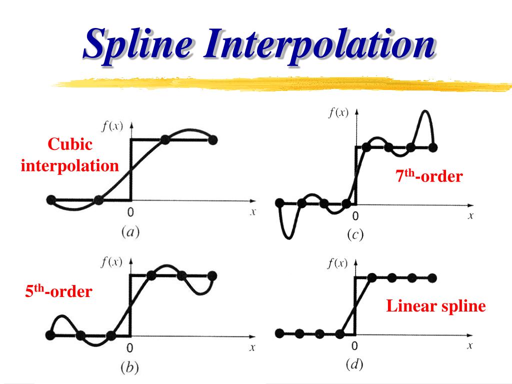
- Forward Curve: Because the spot curve is a single polynomial, the forward curve is also a single, smooth polynomial. However, the oscillations are amplified. Most damningly, the forward curve plummets into negative territory, which implies a clear arbitrage opportunity (you could lock in a risk-free profit). This makes it entirely unsuitable for financial modeling.
C. Cubic Spline Interpolation
- Spot Curve: The cubic spline produces a smooth curve that passes through all data points without the wild oscillations of the single polynomial. It achieves a natural-looking fit that appears economically plausible. This curve is continuous—its first and second derivatives are continuous everywhere.
- Forward Curve: The resulting forward curve is smooth and continuous ( continuity). It stays in positive territory and captures the underlying shape suggested by the data points without introducing spurious volatility or arbitrage opportunities. It represents a stable and believable forecast of future short-term rates.
4. A Framework for Evaluation
The visual evidence is compelling, but for a rigorous comparison, it's useful to evaluate these methods against a set of formal criteria. The following reading from Hagan and West provides an excellent framework for just this purpose.
How To Compare Yield Curve Interpolation Methodologies
This section from "Methods for Constructing a Yield Curve" by Hagan and West outlines the key criteria for judging any yield curve interpolation method.
Read Section 3: "How To Compare Yield Curve Interpolation Methodologies" (page 73). Focus on the criteria listed in points (a), (b), and (c): (a) Quality of the forward rates (positivity, continuity). (b) Locality of the method. (c) Stability of the forwards.
Let's summarize our findings using this framework:
| Criterion | Linear Interpolation | Polynomial Interpolation | Cubic Spline Interpolation |
|---|---|---|---|
| Spot Curve Smoothness | (Continuous) | (Smooth) | (Smooth) |
| Forward Curve Quality | Discontinuous, piecewise constant. | Smooth, but can be wildly oscillating and negative. | Continuous and smooth (). Economically plausible. |
| Locality | Excellent. A change to one point only affects the two adjacent intervals. | Very Poor. A change to one point affects the entire curve. | Good. A change to one point has a localized, decaying impact. |
| Stability / Risk of Oscillation | Excellent. No oscillation. | Very Poor. High risk of Runge's phenomenon. | Good. Stable and non-oscillatory. |
| Overall Suitability | Poor due to discontinuous forwards. | Unsuitable due to oscillations, negative rates, and poor locality. | Excellent. The best trade-off between smoothness and stability. |
This comparison clarifies that while a single high-degree polynomial is "smoother" in a purely mathematical sense ( vs ), its global nature and tendency to oscillate make it a poor choice. Linear interpolation is local and stable but fails on the crucial requirement of a continuous forward curve. Cubic splines emerge as the superior method by providing sufficient smoothness () to guarantee well-behaved forward rates while retaining the local and stable properties of a piecewise approach.
For a deeper dive into the mathematics and visual examples of these failures, you can explore the following resource.
An investigation into popular methods for constructing yield curves
This dissertation provides a thorough analysis of traditional interpolation methods.
I recommend skimming these sections to reinforce what you've seen in the code and plots: Section 4.1 Linear Interpolation (pages 25-29): Look at the equations deriving the forward rate and Figure 4.1, which graphically shows the discontinuous forward curves, including one that turns negative. Section 4.2 Cubic Interpolation (pages 29-34): See the discussion on how even standard cubic splines can lead to issues like negative forward rates (see Figure 4.2). This highlights why more advanced spline methods (like the monotone convex method discussed later in the paper) were developed to guarantee positivity, although the natural spline often performs well in practice. Section 7.1 Locality (pages 57-60): Figure 7.1 provides a powerful visual for the concept of locality. It shows how changing one data point ("blipping" the curve) has a global, rippling effect for a natural cubic spline, whereas more local methods contain the impact. Chapter 8 Conclusions (pages 70-72): This provides a concise summary of the findings, reiterating the flaws of linear and "traditional" cubic methods.
Conclusion
In this lesson, we synthesized our knowledge of different interpolation techniques by conducting a direct, practical comparison. By applying linear, polynomial, and cubic spline interpolation to the same dataset, we have seen firsthand why the choice of method is not arbitrary but has profound implications for the validity of the resulting yield curve.
Key Takeaways:
- Linear Interpolation is simple and stable but fails by producing discontinuous, economically implausible forward rate curves.
- Polynomial Interpolation is mathematically smooth but suffers from Runge's phenomenon, leading to wild oscillations, poor locality, and the potential for negative forward rates, making it unsuitable for financial applications.
- Cubic Spline Interpolation provides the optimal balance. It is smooth enough () to generate continuous and well-behaved forward curves () while being a local method that avoids the instability of high-degree polynomials.
You have now completed the journey from discrete bond prices to a fully constructed, continuous yield curve. You not only know the "how" (bootstrapping and interpolation) but also the critical "why" behind the choice of methodology.
In our next module, we will put this powerful tool to work. We will integrate bootstrapping and spline interpolation into a single workflow to build spot, forward, and par-yield curves from raw market data and, crucially, learn to interpret the economic signals embedded in their shapes.