Interpreting GLM Output

Your Roadmap: The GLM Summary Output

When you fit a GLM and ask for a summary, you get a block of text packed with information. It can be intimidating at first, but it follows a consistent structure. The image below provides an excellent, annotated roadmap of what we'll be covering.

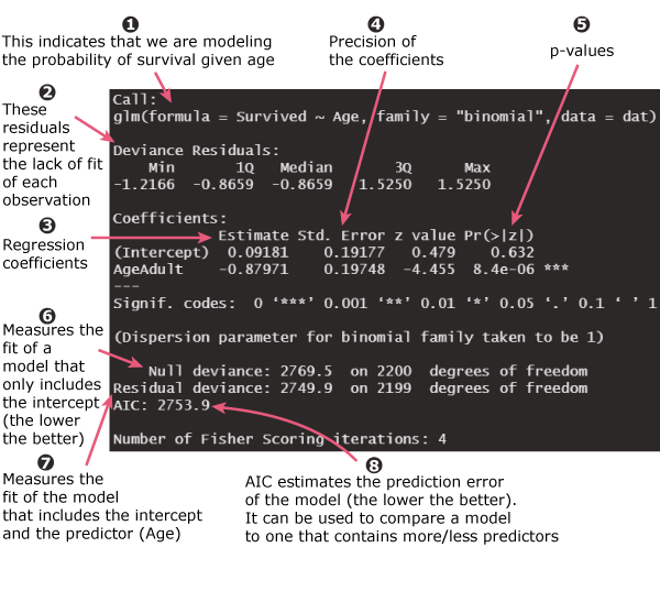
We will work through this output systematically, starting with the most important part: the coefficients table.

Deconstructing the Coefficients Table

The heart of the model summary is the table of coefficients. This is where you find out the direction, magnitude, and statistical significance of your predictors' effects.

To get a feel for how to interpret this table, let's watch a short video. It uses a GLM with a Gaussian family (similar to a standard linear model) which makes the initial interpretation of coefficients as 'slopes' very intuitive. It also does an excellent job of explaining how categorical predictors are handled.

As the video demonstrates, this table contains several key columns:

1. Estimate: This is the coefficient ($\hat{\beta }$), our model's best guess for the relationship between a predictor and the outcome. Crucially, its interpretation depends on the GLM's link function.
2. Std. Error: This measures the precision of the coefficient estimate. A smaller standard error means we are more confident in our estimate.
3. z value (or t value): This is the Wald test statistic. It's calculated as Estimate / Std. Error and tells us how many standard errors the estimated coefficient is from zero.
4. Pr(>|z|): This is the p-value for the Wald test. It answers the question: "If the true coefficient were zero, how likely would we be to see an estimate this far from zero (or further)?" A small p-value (e.g., < 0.05) suggests the predictor has a statistically significant relationship with the outcome.

Interpreting Coefficients: It's All About the Link Function

The most important and nuanced part of interpreting a GLM is understanding that the Estimate is on the scale of the link function, not the original response variable.

Case 1: Logistic Regression (Logit Link)

In logistic regression, the logit link models the logarithm of the odds of the outcome.

• A coefficient ${\beta }_j$ represents the change in the log-odds of the outcome for a one-unit increase in the predictor $x_j$.
• To make this more intuitive, we often exponentiate the coefficient, $e^{{\beta }_j}$, to get an odds ratio.

Let's watch a classic explanation of this from StatQuest.

Case 2: Poisson Regression (Log Link)

In Poisson regression, the log link models the logarithm of the expected count or rate.

• A coefficient ${\beta }_j$ represents the change in the log of the mean count for a one-unit increase in the predictor $x_j$.
• Exponentiating the coefficient, $e^{{\beta }_j}$, gives us a rate ratio. It tells us the multiplicative factor by which the mean count changes for a one-unit increase in the predictor.

To see this in action, let's look at a textual resource.

Understanding Model Fit Statistics

Beyond the coefficients, the summary output provides statistics that help you assess the overall model.

Let's summarize the key terms from that reading:

• Deviance Residuals: These are the GLM equivalent of the residuals you know from linear regression. As a quick diagnostic check, you want to see them distributed roughly symmetrically around a median near zero. A skewed distribution can indicate a poor model fit.

• Null Deviance: This measures the "badness of fit" of an "intercept-only" model (a model with no predictors). It serves as a baseline. The degrees of freedom are $n-1$, where $n$ is the number of observations.

• Residual Deviance: This measures the "badness of fit" of your model, with all its predictors. The degrees of freedom are $n-p-1$, where $p$ is the number of predictors. A model that fits well will have a residual deviance that is significantly smaller than the null deviance.

• AIC (Akaike Information Criterion): AIC is a metric used for model comparison. It balances model fit (how well it explains the data) with model complexity (how many predictors it uses). Its absolute value is not interpretable, but when comparing several different models, the one with the lower AIC is generally preferred.

Conclusion

You've now learned how to navigate and interpret the standard summary of a Generalized Linear Model. You can deconstruct the output into its fundamental parts and understand what each number is telling you about your model and your data.

Key Takeaways:

• The coefficients table is the core of the output, providing estimates, standard errors, and Wald test results (z-values and p-values) for each predictor.
• Coefficient interpretation is link-dependent: In logistic regression, estimates are log-odds, and in Poisson regression, they are log-rates. Exponentiating them yields more interpretable odds ratios and rate ratios.
• Categorical predictor coefficients represent the difference relative to a baseline (reference) category.
• Deviance (Null and Residual) provides a measure of how well the model fits compared to a baseline, while AIC is a crucial tool for comparing competing models.
• The p-values in the summary table come from Wald tests, and as we learned previously, they should be interpreted with some caution, especially if they are borderline significant.

Preview of the Next Lesson:

In this lesson, we introduced the concept of deviance as a measure of model fit. In our next session, we will go much deeper. We will learn how to formally assess the overall goodness of fit of a model using deviance-based statistics and the goodness-of-fit chi-squared test. This will allow us to move from simply comparing models with AIC to making an absolute judgment about whether our chosen model is a good representation of the data.