Deviance and Goodness-of-Fit

The Logic of Deviance: Comparing to Perfection

To understand a goodness-of-fit test, we first need a benchmark for a "perfect" fit. In GLMs, this benchmark is the saturated model.

A saturated model is a model that is so complex it fits the data perfectly. It achieves this by having one parameter for every unique combination of predictor values in your data. It essentially "memorizes" the dataset. While it provides a perfect fit to the existing data, it's useless for generalization or prediction, so we don't use it as our final model. However, it serves as the ideal standard against which we measure our own, more parsimonious model.

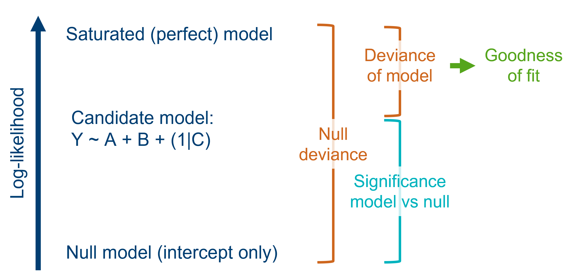
The residual deviance that we saw in the last lesson is a measure of the "distance" between the log-likelihood of our model and the log-likelihood of this perfect saturated model.

To build a strong intuition for this, let's watch a segment from StatQuest.

The key idea is that a smaller residual deviance means our model's fit is closer to the "perfect" fit of the saturated model. The goodness-of-fit test formally asks: "Is our model's deviance small enough to be considered a good fit, or is it so large that we must conclude our model is inadequate?"

The diagram below visualizes this relationship. The residual deviance (labeled "Deviance of model") is the gap between the log-likelihood of the saturated model and your candidate model.

The Goodness-of-Fit Test using Deviance

The residual deviance is not just a descriptive number; it's a test statistic. We can use it to conduct a formal hypothesis test.

• Null Hypothesis ($H_0$): The current model fits the data adequately.
• Alternative Hypothesis ($H_a$): The current model does not fit the data adequately (there is a significant "lack of fit").

Under the null hypothesis (and subject to some important conditions we'll discuss next), the residual deviance follows a chi-squared (${\chi }^2$) distribution.

The degrees of freedom ($df$) for this test are calculated as:

where:

• $n$ = the number of unique covariate patterns in the data.
• $p$ = the number of parameters in your model (including the intercept).

To perform the test, we compare our model's residual deviance to a ${\chi }^2$ distribution with $n-p$ degrees of freedom. A large deviance value will result in a small p-value. If this p-value is below our significance threshold (e.g., 0.05), we reject $H_0$ and conclude that the model does not fit the data well.

Let's ground this with a concise reading.

Notice a key rule of thumb: for a good-fitting model, we expect the residual deviance to be close to its degrees of freedom. If Residual Deviance >> df, it's a strong signal of lack of fit.

A Critical Caveat: When the Deviance GOF Test Fails

This is arguably the most important practical point of the lesson. The chi-squared approximation for the deviance distribution only holds for grouped data where expected counts are sufficiently large.

• Grouped Data: This refers to datasets where multiple individuals share the same set of predictor values. For each unique covariate pattern, you have a count of successes ($y_i$) and failures ($n_i-y_i$). The rrHale.df data from the resource LINK (with NumVotes per county) is an example of grouped data.
• Ungrouped Data: This is common in logistic regression where the outcome is binary (0/1) for each individual, and many individuals have unique predictor values (especially with continuous predictors like age or BMI). Here, the number of trials for each "group" is just 1.

For ungrouped data, the residual deviance does NOT follow a ${\chi }^2$ distribution, and the GOF test described above is invalid.

Let's see the dramatic effect this has.

The Alternative: The Hosmer-Lemeshow Test

So, what do you do when you have ungrouped data or models with continuous predictors? The most common alternative is the Hosmer-Lemeshow (H-L) test.

The H-L test has the same hypotheses as the deviance GOF test, but it works differently:

1. It takes all of your observations and sorts them based on their predicted probability from your model.
2. It then divides the data into a number of groups (typically 10, forming "deciles of risk").
3. Within each group, it compares the observed number of successes to the number of successes your model predicted (by summing the predicted probabilities).
4. It computes a chi-squared statistic based on the differences between observed and expected counts across all groups.

A non-significant p-value (e.g., p > 0.05) is what you want, as it indicates no significant difference between the observed and predicted outcomes, suggesting a good model fit.

Conclusion

You've now learned how to move beyond interpreting individual coefficients to assessing the absolute, overall fit of your GLM. This is a critical checkpoint before you can confidently report or use a model.

Key Takeaways:

• A goodness-of-fit (GOF) test assesses whether your model as a whole is an adequate description of the data. The null hypothesis is that the model fits well.
• The residual deviance acts as a test statistic, comparing your model to a theoretically perfect saturated model.
• For grouped data with large enough counts, the residual deviance follows a ${\chi }^2$ distribution, and a large deviance relative to its degrees of freedom indicates a lack of fit.
• Crucially, this test is invalid for ungrouped binary data or models with continuous predictors, as the deviance no longer approximates a ${\chi }^2$ distribution.
• For these common cases, the Hosmer-Lemeshow test is the appropriate alternative for assessing goodness-of-fit.

Preview of the Next Lesson:

A good GOF test result tells us the model fits well on average. But what if it fits most data points well, while a few specific points are predicted very poorly? These outliers or influential points can distort our model. In the next lesson, we will learn how to perform residual diagnostics to zoom in and examine the fit at the individual observation level.