Residual Analysis for Model Diagnostics

Residuals in GLMs: More Than Just "Observed - Predicted"

In ordinary linear regression, a residual is simply the difference between the observed value ($y_i$) and the predicted value (${\hat{y}}_i$). In the GLM world, it's a bit more complex. Because our response variable isn't assumed to have constant variance (e.g., in Poisson or Binomial models), we need more sophisticated ways to measure the error for each point.

We will focus on two main types of residuals for GLMs: Pearson residuals and deviance residuals.

Let's start with deviance residuals, as they connect directly to our last lesson. Remember that the total residual deviance measured the overall lack of fit. A deviance residual is simply the contribution of a single data point to that total.

While deviance residuals are excellent for spotting general patterns of misfit, Pearson residuals are defined slightly differently. They are scaled by the estimated standard deviation of the response variable at each point. This makes them particularly useful for checking if our assumption about the variance function is correct.

In practice, we often use standardized versions of these residuals. Standardization adjusts the residuals to have a more constant variance and accounts for leverage (which we'll define shortly), making it easier to spot outliers.

For a formal definition of these different residual types, please review the following text.

Using Residual Plots to Diagnose Model Misspecification

Once we have our residuals, we can create diagnostic plots to look for signs of trouble. The goal in all these plots is to see a random, patternless cloud of points scattered around zero. Any systematic pattern is a red flag.

Here are the most important plots and what they help us diagnose:

1. Residuals vs. Fitted Values (or Linear Predictor):

   • What it checks: The correctness of the systematic part of the model (link function) and the variance function.
   • What to look for:
     • Curvature: A U-shape or S-shape suggests you may have chosen the wrong link function or missed a quadratic term for a predictor.
     • A "funnel" shape: If the spread of residuals increases or decreases as the fitted value changes, your variance function is likely incorrect (e.g., you assumed Poisson variance when the data is overdispersed).

2. Residuals vs. Explanatory Variables:

   • What it checks: Whether the relationship with a specific predictor is modeled correctly.
   • What to look for: Curvature in a plot of residuals against a predictor x indicates that the functional form of x is wrong. You might need to transform it (e.g., use log(x)) or add a polynomial term (x^2).

3. Absolute Residuals vs. Fitted Values:

   • What it checks: This plot is a more direct way to assess the variance function.
   • What to look for: A trend in this plot indicates the variance is not behaving as your model assumes. A positive trend suggests the variance grows faster than you modeled.

The following reading provides a great summary of these and other useful diagnostic plots.

A Modern Approach: The DHARMa Package

Manually creating and interpreting all these plots can be tedious. In R, the DHARMa package provides a fantastic, unified framework for GLM diagnostics by simulating new data from your fitted model and comparing it to your observed data.

Identifying Outliers and Influential Points

The second major goal of diagnostics is to find individual points that are either poorly explained by the model or have a disproportionately large impact on it.

Three concepts are key here:

• Outlier: An observation with a response value ($y_i$) that is unusual given its predictor values ($x_i$). These points will have large residuals. Studentized residuals are typically used to formally identify them.
• Leverage: An observation with an unusual combination of predictor values ($x_i$). Such a point is far from the center of the predictor space and has the potential to be influential. Leverage is measured by hat-values ($h_i$).
• Influence: The "damage" a single point does to your model. An influential observation is one that, if removed, would cause a substantial change in the estimated coefficients. Influence is a combination of being an outlier and having high leverage. The most common measure is Cook's Distance.

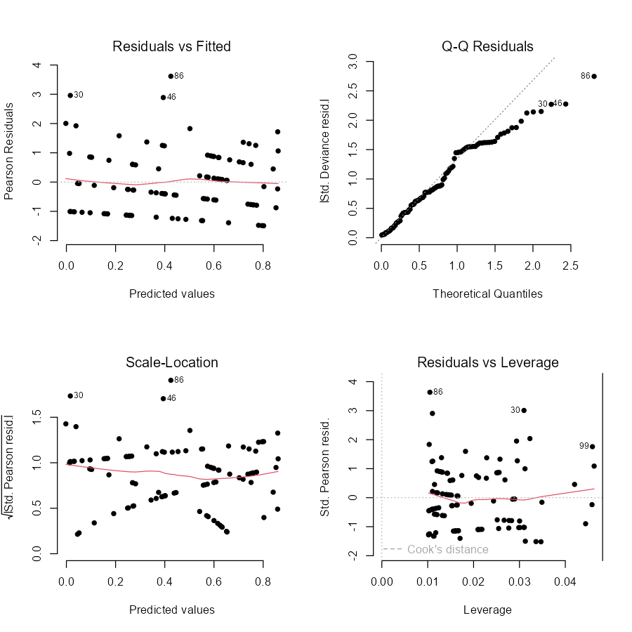
The workflow is to identify points with high leverage or high Cook's Distance and investigate them. Does the data point represent a data entry error? Or is it a genuinely unusual case that might warrant special attention or even removal from the dataset before finalizing the model?

Conclusion

Model assessment is a two-step process. First, you check the overall goodness-of-fit to see if the model is plausible on a macro level. Then, you must perform residual diagnostics to ensure it's behaving well on a micro level.

Key Takeaways:

• Residuals in GLMs (like Pearson and deviance residuals) are more complex than in linear regression because they must account for non-constant variance.
• Plotting residuals against fitted values and predictors helps diagnose model misspecification, such as an incorrect link function or the need to transform a predictor. A patternless, random cloud of points is the ideal.
• Leverage (measured by hat-values) identifies points with unusual predictor values that have the potential to be influential.
• Influence (measured by Cook's Distance) identifies points that, if removed, would significantly change your model's coefficients. These are the most problematic points and require investigation.

Preview of the Next Lesson:

We have now completed our tour of the foundations of Generalized Linear Models! We've covered the core components, how to perform inference on coefficients, and how to assess model fit. In the next module, we will put all this theory into practice by focusing on the most famous GLM of all: Binary Logistic Regression. We'll learn how to formulate the model, interpret its coefficients in terms of odds ratios, and apply the diagnostic techniques you've learned here.