Binary Logistic Regression: Model Formulation and Logit Interpretation

Why Ordinary Linear Regression Fails for Binary Outcomes

Let's start with a foundational question. You have a good understanding of linear regression. Why can't we just apply it when our dependent variable, $Y$, can only be 0 or 1?

There are several critical problems with this approach.

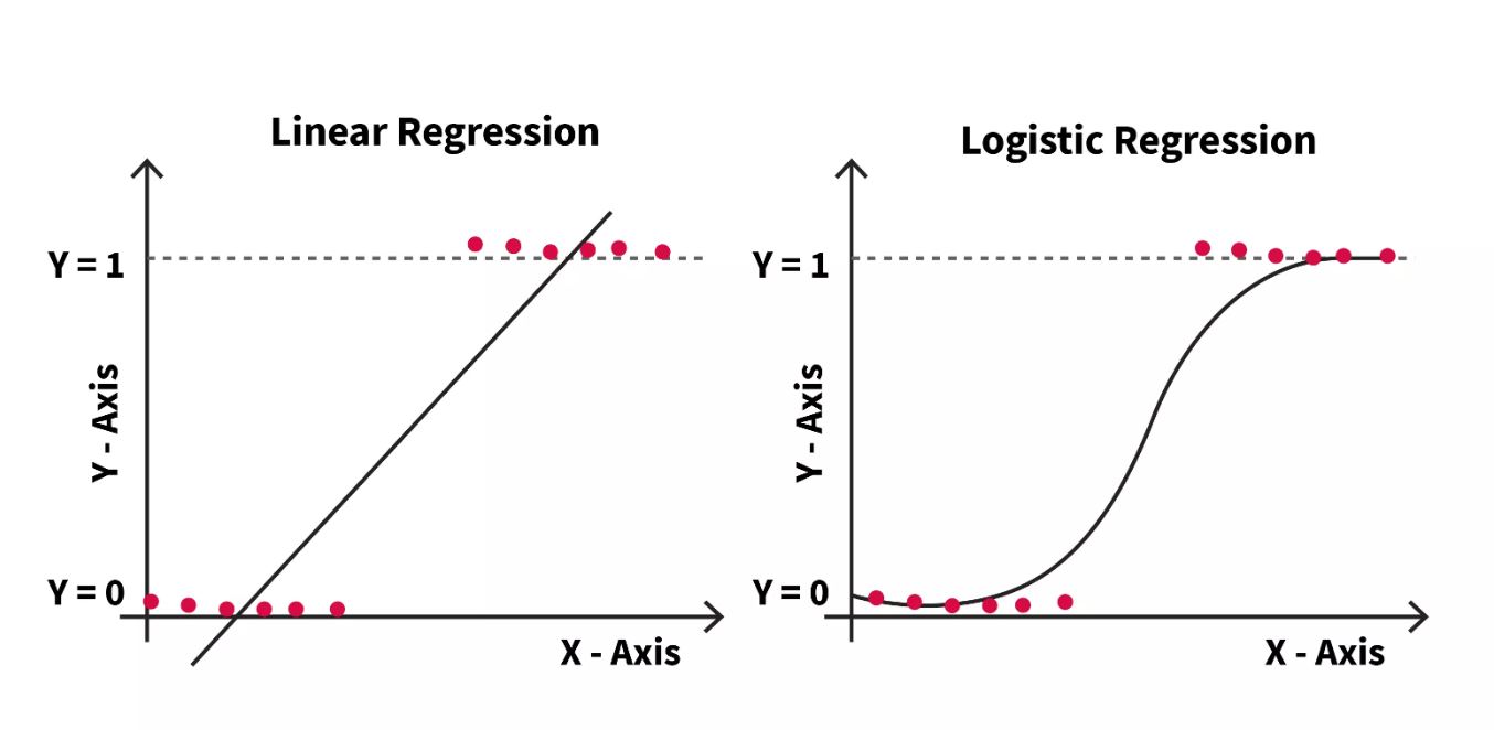
As the image on the left shows, a simple linear model (Y = a + bX) will try to fit a straight line through data points clustered at Y=0 and Y=1. This leads to major issues:

1. Impossible Predictions: The line will inevitably predict values above 1 and below 0. How do you interpret a probability of 1.2 or -0.1? It's meaningless.
2. Incorrect Functional Form: The true relationship between a predictor and a probability is rarely linear. Often, a small change in a predictor has a large effect in the middle of its range but a smaller effect at the extremes. This suggests an "S-shaped" curve, not a straight line.
3. Violation of Core Assumptions: The assumptions of linear regression, such as normally distributed and homoscedastic (constant variance) errors, are violated when the outcome is binary.

To get a solid grasp of these failures, please read the first part of the following document.

The Solution: Modeling a Transformation of the Probability

The core problem is that the linear predictor, ${\beta }_0+{\beta }_{1}X$, is unbounded (it can go from $-\infty$ to $+\infty$), while the outcome we want to predict, a probability $\pi$, is bounded between 0 and 1.

The solution is to find a function that can "stretch" the [0, 1] interval to cover the entire number line. This transformation is called the logit link function. It's a two-step process.

Step 1: From Probability to Odds

Instead of modeling the probability $\pi$ directly, we can model the odds.

The odds represent the ratio of the probability of success to the probability of failure.

• If $\pi =0.5$, the odds are 1 (or "1 to 1").
• If $\pi =0.8$, the odds are $0.8/0.2=4$ (or "4 to 1").
• As $\pi$ approaches 1, the odds approach $+\infty$.
• As $\pi$ approaches 0, the odds approach 0.

By converting to odds, we've solved half the problem: we've removed the upper bound of 1. The range is now $[0,+\infty )$.

Step 2: From Odds to Log-Odds (the Logit)

To remove the lower bound of 0, we simply take the natural logarithm of the odds. This gives us the log-odds, which is also called the logit.

The range of the log-odds is $(-\infty ,+\infty )$. This is exactly what we needed! We now have a quantity that is unbounded, just like our linear predictor.

The following video provides an excellent visual and conceptual walkthrough of this transformation.

Formulating the Binary Logistic Regression Model

Now we can formally define the model. Binary logistic regression is a GLM where:

1. Random Component: The response variable $Y_i$ for a given set of predictors follows a Binomial distribution. For a single observation, this is a Bernoulli distribution (a single trial with probability of success ${\pi }_i$).
2. Systematic Component: The predictors are combined linearly to form the linear predictor, ${\eta }_i={\beta }_0+{\beta }_1{x}_{i1}+\cdots +{\beta }_k{x}_{ik}$.
3. Link Function: The logit function links the expected value of the response, $E(Y_i)={\pi }_i$, to the linear predictor.

Putting it all together, the logistic regression model is:

This equation states that the log-odds of success is a linear function of the predictors. This is the fundamental equation you need to understand.

By rearranging the formula, we can express the probability ${\pi }_i$ as a function of the predictors. This S-shaped function is sometimes called the logistic function or sigmoid function.

The following reading provides a slightly more formal summary of these components and presents the model in the context of the GLM framework we've already learned.

A First Look at Interpreting Coefficients

So what do the $\beta$ coefficients in our model equation actually mean? Since the left side of the equation is in log-odds, the coefficients must also be interpreted on that scale.

• ${\hat{\beta }}_0$ (the intercept) is the estimated log-odds of success when all predictor variables are zero.
• ${\hat{\beta }}_1$ is the estimated change in the log-odds for a one-unit increase in the predictor $x_1$, holding all other predictors constant.

Let's return to the StatQuest video, which provides a simple, clear example of this interpretation for both continuous and categorical predictors.

While interpreting coefficients as changes in log-odds is technically correct, it's not very intuitive. In our next lesson, we will focus entirely on the much more practical skill of converting these log-odds back into odds ratios, which are far easier to understand and explain.

Conclusion

This lesson established the "why" and "what" of binary logistic regression. We've seen that it's not just an arbitrary choice but a necessary and elegant solution to the problems that arise when trying to model binary outcomes.

Key Takeaways:

• Ordinary Linear Regression is unsuitable for binary (0/1) outcomes because it can produce impossible predictions and violates key statistical assumptions.
• Logistic regression solves this by modeling a transformation of the probability, not the probability itself.
• The logit link function, $\log (\pi /(1-\pi ))$, transforms a probability (bounded at 0 and 1) into log-odds (unbounded), which can then be modeled as a linear combination of predictors.
• The fundamental logistic regression equation is $\text{logit}({\pi }_i)={\beta }_0+{\beta }_1{x}_i$, which states that the log-odds of the outcome is a linear function of the predictors.
• The model coefficients ($\beta$'s) represent changes in the log-odds of the outcome.

Preview of the Next Lesson:

We've learned that coefficients are on the log-odds scale. Now, how do we make them interpretable for a report or a stakeholder? In the next lesson, we will focus on interpreting logistic regression coefficients. You will learn how to convert the raw coefficients into odds ratios, attach confidence intervals to them, and explain precisely what they mean in a practical context.