Interpreting Logistic Regression Coefficients

Hello! Welcome back.

In our last lesson, we established the core structure of the binary logistic regression model. We learned that to model a binary outcome, we model the log-odds of that outcome as a linear function of the predictors:

lo g (\frac{π}{1 - π}) = β_{0} + β_{1} x_{1} + \dots + β_{k} x_{k}

This means that a coefficient, like $β_{1}$ , represents the change in the log-odds of the outcome for a one-unit increase in the predictor $x_{1}$ . While this is technically correct, "log-odds" are not intuitive for most people to understand or explain.

Today, we will focus on translating these coefficients into a much more practical and interpretable metric: the odds ratio (OR). By the end of this lesson, you will be able to take the output from a logistic regression model, convert the coefficients into odds ratios, and confidently interpret what they mean, complete with confidence intervals.

The Fundamental Link: From Log-Odds to Odds Ratios

The key to making logistic regression coefficients interpretable lies in a simple mathematical operation: exponentiation. Let's see why this works.

Consider a simple model with one predictor, $x$ :

lo g (odds) = β_{0} + β_{1} x

Now, let's compare the odds for two scenarios: one where the predictor has a value of $x$ , and another where it has a value of $x + 1$ .

Log-odds at $x + 1$ : $lo g (odds_{x + 1}) = β_{0} + β_{1} (x + 1)$
Log-odds at $x$ : $lo g (odds_{x}) = β_{0} + β_{1} x$

If we subtract the second equation from the first, we get the change in the log-odds for a one-unit increase in $x$ :

lo g (odds_{x + 1}) - lo g (odds_{x}) = (β_{0} + β_{1} x + β_{1}) - (β_{0} + β_{1} x) = β_{1}

Using the logarithm rule $lo g (a) - lo g (b) = lo g (a / b)$ , we can rewrite the left side:

lo g (\frac{odds _{x + 1}}{odds _{x}}) = β_{1}

The term inside the logarithm, $\frac{odds _{x + 1}}{odds _{x}}$ , is the odds ratio. It's the ratio of the odds at one value of the predictor compared to the odds at another value one unit lower.

To isolate the odds ratio, we simply exponentiate both sides of the equation:

Odds Ratio (OR) = exp (β_{1}) = e^{β_{1}}

This elegant relationship is the cornerstone of interpreting logistic regression coefficients. The following article provides a concise mathematical derivation that reinforces this key concept.

A Deeper Dive into Odds Ratios Using Logistic Regression

The article 'A Deeper Dive into Odds Ratios Using Logistic Regression' clearly shows the mathematical steps to get from the logit function to the odds ratio.

Please read the section 'From Logit to Odds Ratio'. Focus on how dividing the odds for an exposed group (x=1) by the odds for an unexposed group (x=0) results in the odds ratio being the exponential of the coefficient β1.

Interpreting the Odds Ratio

Now that we know $OR = e^{β}$ , how do we interpret it? An odds ratio tells you how the odds of the outcome change multiplicatively for a one-unit change in the predictor variable, holding all other variables constant.

If $β > 0$ , then $OR > 1$ : The odds of the outcome increase as the predictor increases.
If $β < 0$ , then $OR < 1$ : The odds of the outcome decrease as the predictor increases.
If $β = 0$ , then $OR = 1$ : The predictor has no effect on the odds of the outcome.

Let's look at how this plays out for different types of predictors.

Case 1: Binary Predictor

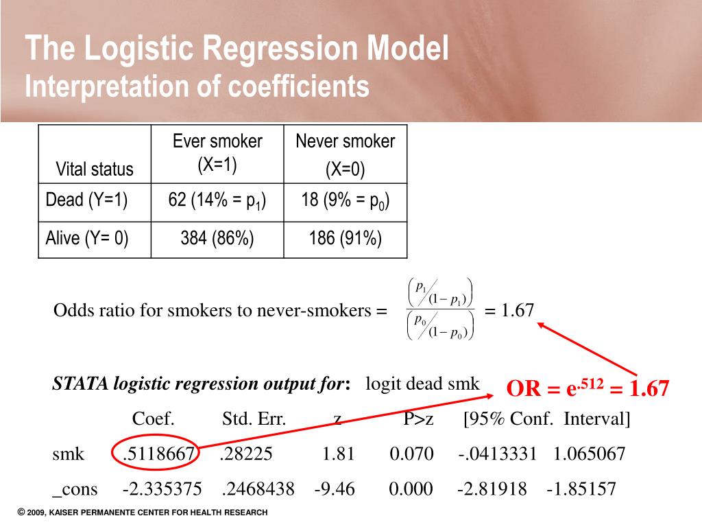
This is the most straightforward case. A binary predictor is typically coded as 0 and 1 (e.g., non-smoker=0, smoker=1). The odds ratio, $e^{β}$ , directly compares the odds of the outcome for the group coded as 1 to the group coded as 0.

Example: A study models the odds of death. The predictor smoker is 1 for smokers and 0 for non-smokers. The fitted model gives a coefficient for smoker of $β^_{smoker} = 0.693$ .

The odds ratio is $e^{0.693} \approx 2.0$ .

Interpretation: The odds of death for smokers are 2.0 times the odds of death for non-smokers.

The image below provides a fantastic visual link between a simple 2x2 contingency table, the odds ratio calculated from it, and the exponentiated coefficient from a logistic regression model run on the same data.

Logistic Regression Coefficient Interpretation and Odds Ratio — This image shows that the odds ratio for dying (smoker vs. never-smoker) calculated from a 2x2 table (3.125) is the same as the exponentiated coefficient for the smoking variable from a logistic regression output (e^1.13943 = 3.125).

Case 2: Continuous Predictor

For a continuous predictor (like age or income), the interpretation is for a one-unit increase.

Example: A model predicts the probability of being approved for a mortgage based on credit_score. The coefficient for credit_score is $β^_{score} = 0.015$ .

The odds ratio is $e^{0.015} \approx 1.015$ .

Interpretation: For each one-point increase in credit score, the odds of being approved for a mortgage increase by a factor of 1.015 (or about 1.5%), holding other factors constant.

The following video walks through the interpretation of both raw coefficients (log-odds) and odds ratios for continuous and categorical predictors using a practical example.

Interpreting Odds Ratios in Logistic Regression

This video from Simplistics (QuantPsych) does an excellent job of explaining the mental gymnastics required to interpret logistic regression output. It contrasts the unintuitive log-odds with the more practical odds ratios.

Please watch from 12:03 to 18:07 and then from 19:51 to 21:12. The first part covers the interpretation for a continuous predictor (willpower), and the second part covers a categorical predictor (superhero status). Focus on how the narrator translates the numerical odds ratio into a sentence.

Confidence Intervals for Odds Ratios

A point estimate for an odds ratio is useful, but a confidence interval (CI) is better because it quantifies our uncertainty. When you fit a model, the software provides a CI for the coefficient $β$ . To get the CI for the odds ratio, you simply exponentiate the lower and upper bounds of the coefficient's CI.

If the 95% CI for $β$ is $[β_{lower}, β_{upper}]$ , then the 95% CI for the OR is $[exp (β_{lower}), exp (β_{upper})]$ .

The interpretation of this interval is crucial for hypothesis testing. If the 95% CI for an odds ratio does not contain the value 1, the effect is statistically significant at the 0.05 level. This is because an OR of 1 implies no effect.

The following resource provides a very direct, practical example of how to do this in R.

R: How to Calculate Odds Ratios in Logistic Regression Model

This article from Statology shows the exact R code to fit a logistic regression model and then immediately compute the odds ratios and their confidence intervals.

Read through the page, focusing on the example section. Pay attention to the glm() function to fit the model and then the exp(coef(model)) and exp(confint(model)) syntax to get the odds ratios and their confidence intervals. Notice the final interpretation provided for the 'balance' variable.

If you work primarily in Python, the article "A Deeper Dive into Odds Ratios" (resource LINK), which you looked at earlier, also demonstrates this process using the statsmodels library in the section titled "Getting the odds ratio and its confidence interval".

A Deeper Look: Odds Ratios for Any Interval

So far, we've interpreted the OR for a one-unit change in a continuous predictor. But what if a one-unit change isn't meaningful? For example, what is the effect of a 10-year increase in age, not just one year?

The relationship $OR = e^{β}$ is elegantly scalable. The odds ratio for a c-unit increase in a predictor $x$ is given by:

OR_{c-unit change} = exp (c \times β)

Example: Let's go back to our mortgage example, where $β^_{score} = 0.015$ . What is the odds ratio for a 50-point increase in credit score?

OR_{50-point change} = exp (50 \times 0.015) = exp (0.75) \approx 2.12

Interpretation: A 50-point increase in credit score is associated with a 2.12 times increase in the odds of being approved for a mortgage.

The following video is entirely dedicated to this concept and provides an exceptionally clear explanation, showing how a single coefficient can be used to calculate the odds ratio for any interval of interest.

Statistics 101: Logistic Regression, Odds Ratio for Any Interval

This Brandon Foltz video provides an in-depth, step-by-step guide to calculating odds ratios for any interval. It powerfully demonstrates the exponential relationship between the change in a predictor and the corresponding odds ratio.

Watch from 13:37 to 20:20. The video graphs the odds ratio against the change in the predictor, revealing an exponential curve. The key insight comes when it shows that the parameter of this curve is precisely the model's beta coefficient. This is a powerful demonstration of how the model works.

Conclusion

You have now learned the essential skill of making logistic regression results interpretable and meaningful. Moving from abstract log-odds to concrete odds ratios allows you to communicate your findings effectively to any audience.

Key Takeaways:

Logistic regression coefficients ( $β$ ) represent the change in the log-odds of an outcome.
To make them interpretable, we exponentiate them to get the odds ratio (OR): $OR = e^{β}$ .
The OR is the multiplicative change in the odds of the outcome for a one-unit increase in the predictor.
For a c-unit increase in a predictor, the OR is calculated as $exp (c \times β)$ .
The confidence interval for an OR is found by exponentiating the CI of the corresponding $β$ . If this interval does not include 1, the effect is statistically significant.

Preview of the Next Lesson:

We can now build a logistic regression model and interpret its coefficients. But how do we know if the model is any good? Is it a good fit for the data? In our next lesson, we will cover methods for assessing the goodness of fit of a logistic regression model, including deviance-based statistics and the Hosmer-Lemeshow test.

Recommended resources