Assessing Logistic Regression Fit: Deviance and Hosmer-Lemeshow

What is Goodness of Fit?

It's crucial to distinguish between two ways of evaluating a model:

1. Measures of Predictive Power: These tell you how well the model predicts the outcome. We'll cover metrics like the Area Under the ROC Curve (AUC) in a future lesson. A model can have low predictive power but still be a "good fit."
2. Goodness-of-Fit (GOF) Tests: These are formal hypothesis tests where the null hypothesis ($H_0$) is that the model is correctly specified and fits the data well. A non-significant result (high p-value) is what we want, as it indicates no evidence of a poor fit.

A model with low predictive power might simply reflect a reality where the outcome is hard to predict. However, a model that fails a GOF test suggests that the underlying mathematical assumptions are wrong—for example, a linear relationship was assumed when a curved one was needed. The paper below by Paul Allison gives an excellent introduction to this distinction.

Assessing Fit with Deviance

In linear regression, you are familiar with the Residual Sum of Squares (RSS) as a measure of how far the data points are from the fitted regression line. A smaller RSS indicates a better fit.

In logistic regression, the equivalent concept is deviance. Deviance is derived from the model's log-likelihood and serves the same purpose: a lower deviance indicates a better fit to the data.

The Null, Proposed, and Saturated Models

To use deviance effectively, we compare our model against two benchmarks:

• Null Model: The simplest model, containing only an intercept. It predicts the same probability (the overall sample proportion) for every observation. This represents the worst-case scenario, our baseline. Its deviance is called the Null Deviance.
• Proposed Model: This is the model you have actually fitted, with your chosen predictors. Its deviance is often called the Residual Deviance.
• Saturated Model: A hypothetical, perfect model with one parameter for every data point. It fits the data perfectly. This represents the best-case scenario. For logistic regression with ungrouped binary data, its log-likelihood is 0, which means its deviance is also 0.

The StatQuest video below provides a brilliant conceptual overview of these three models and how deviance is used to compare them.

Using Deviance in Practice

There are two primary ways we use deviance statistics:

1. Comparing Nested Models (Likelihood Ratio Test)

The difference in deviance between two nested models (where one is a simpler version of the other) follows a chi-square distribution. This is known as the Likelihood Ratio Test.

The test statistic is $G^2=\text{Deviance(Reduced Model)}-\text{Deviance(Full Model)}$.
The degrees of freedom are the difference in the number of parameters between the two models.

For example, to test the overall significance of your model, you can compare your proposed model (full) against the null model (reduced):

A significant p-value here means your model as a whole is a significant improvement over just using the intercept.

2. The Deviance Goodness-of-Fit Test

This test compares your proposed model against the saturated model to assess overall fit. The test statistic is simply the Residual Deviance of your model.

The degrees of freedom are $c-p$, where $c$ is the number of unique combinations of predictor variables (covariate patterns) and $p$ is the number of parameters in your model.

When it fails: This test is only reliable when you have replicated data—that is, multiple observations for each unique covariate pattern. In most modern datasets, especially those with continuous predictors, each observation is its own unique pattern ($c$ is close to the sample size $n$). In such cases, the chi-square approximation is poor, and this test is not valid.

The Hosmer-Lemeshow Test

So, what do we do when the deviance GOF test isn't valid? The Hosmer-Lemeshow (H-L) test was designed specifically for this common scenario.

How It Works (Conceptually)

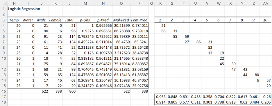
The H-L test uses a clever grouping strategy:

1. Fit your model and get the predicted probability for every observation.
2. Sort the data based on these predicted probabilities, from lowest to highest.
3. Divide the data into $g$ groups of roughly equal size (10 is the standard). This creates "deciles of risk."
4. For each group, compare the observed number of events to the expected number of events (which is the sum of predicted probabilities for that group).
5. A chi-square statistic is calculated from these observed and expected counts. The degrees of freedom are $g-2$.

Interpretation

The null hypothesis for the H-L test is that the model fits the data well. Therefore, a high p-value ($>0.05$) is good, indicating no statistical evidence of a poor fit. A low p-value suggests the model is misspecified.

When It Fails: The Problems with the Hosmer-Lemeshow Test

While widely used, the H-L test has several well-documented and serious limitations that you must be aware of for a proper functional understanding.

As you just read, the main problems are:

• Arbitrary Grouping: The test result can change dramatically depending on the number of groups you choose (e.g., 9 vs. 10).
• Counter-intuitive Behavior: Adding a significant variable can sometimes make the fit worse according to the H-L test, and vice-versa.
• Low Power: It may fail to detect certain types of important model misspecification.

Because of these issues, a non-significant H-L test is reassuring but not definitive proof of a good fit. A significant H-L test, however, should be treated as a serious red flag that your model may be misspecified.

Conclusion

You now have the tools to evaluate whether your logistic regression model provides a good fit to your data.

Key Takeaways:

• Goodness of fit assesses if the model's structure is correct, which is distinct from its predictive power.
• Deviance is the key metric for fit in logistic regression, analogous to RSS in linear regression. Lower deviance is better.
• The Deviance Goodness-of-Fit Test (using the residual deviance) is a formal test of fit but is only valid for grouped/replicated data.
• The Hosmer-Lemeshow (H-L) Test is used for the common case of ungrouped data (e.g., with continuous predictors). A high p-value indicates a good fit.
• The H-L test has serious limitations, including sensitivity to the number of groups and low power. It should be interpreted with caution.

Preview of the Next Lesson:

We have focused on assessing the fit of the model's structure. In the next lesson, we will shift gears to assess its performance. We will ask: How well does our model actually distinguish between the two outcomes? To answer this, we will introduce the confusion matrix and derive essential performance metrics like sensitivity and specificity.