Hello! In our last lesson, we introduced the three main tests for GLM coefficients: the Likelihood Ratio Test (LRT), the Wald test, and the Score test. We established the core intuition that they all assess the evidence against the null hypothesis () by examining the log-likelihood function in different ways.
This lesson builds directly on that foundation. Our goal is to move from what these tests are to why they differ and what those differences mean in practice. While the tests give identical results in ordinary linear regression, they diverge in GLMs, and understanding this divergence is key to a functional understanding of model inference. We will compare their theoretical properties and explore practical scenarios where you might get different answers from each test, and most importantly, which one to trust.
Revisiting the Three Perspectives
As a quick refresher, all three tests quantify the "discrepancy" between the maximum likelihood estimate () and the null hypothesis value (, usually 0).
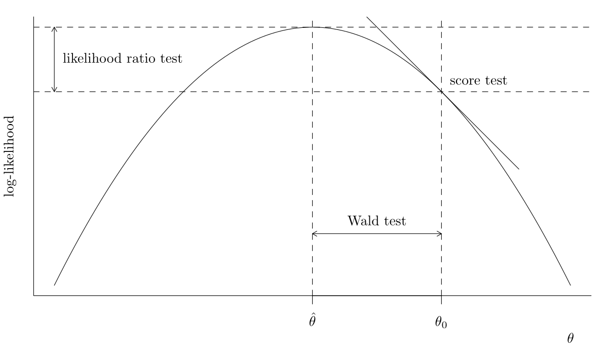
Let's briefly re-watch the video from our last lesson that masterfully visualizes these three approaches.
Wald test | Likelihood ratio test | Score test
The video 'Wald test | Likelihood ratio test | Score test' provides a clear, conceptual overview of the three tests. We'll watch the full video this time to solidify the concepts before diving deeper into their differences.
Please watch the entire video (about 13 minutes). As you watch, pay attention to: The distinct approach of each test (horizontal, vertical, slope). The fact that each test statistic is compared to a chi-squared distribution. The final section (starting around 11:41) which discusses why there are three tests and notes that they converge in large samples—this is the jumping-off point for our lesson today.
Theoretical Differences: Why Aren't They the Same?
The video correctly states that for large samples, the tests converge. This property is called asymptotic equivalence. Their differences arise in finite samples and stem from the specific information each test uses.
1. Invariance to Parameterization
This is perhaps the most important theoretical and practical difference between the tests. A test is "invariant" if its result doesn't change when you re-express the hypothesis. For example, testing if a coefficient is zero () is identical to testing if the odds ratio is one (). A good test should give the same p-value for both.
- Likelihood Ratio Test & Score Test: Are invariant. They produce the same result regardless of how the parameter is expressed. This is a significant strength.
- Wald Test: Is NOT invariant. Because it relies on a quadratic approximation of the log-likelihood function around the MLE, and this approximation changes under non-linear transformations (like exponentiation), you can get different p-values for logically identical hypotheses.
The following reading explains this crucial drawback of the Wald test.
Chapter 19 Inference in Logistic Regression
The text 'Chapter 19 Inference in Logistic Regression' clearly explains the different properties of the LRT and Wald tests, including the critical issue of parameterization.
Please read sections '19.2.1 Likelihood Ratio Test (LRT)' and '19.2.4 Wald Test'. Focus on the advantages and drawbacks listed for each. Specifically, note that the LRT 'doesn’t depend upon the model parameterization,' while the Wald test 'does depend upon the model parameterization.'
This lack of invariance means the Wald test can be less reliable, especially when the shape of the log-likelihood function is far from a perfect parabola, which often happens in smaller samples or with rare outcomes.
Practical Differences: When and How They Disagree
In large samples, the three tests will lead to the same conclusion. In the smaller, messier samples we often encounter in the real world, their results can diverge.
The Inequality: Wald ≥ LRT ≥ Score
For many common models, a useful (though not universal) rule of thumb is that the test statistics follow a predictable inequality:
Wald statistic ≥ Likelihood Ratio statistic ≥ Score statistic
This means that for the same data, the Wald test will produce the largest test statistic (and thus the smallest p-value), making it the most likely to reject the null hypothesis. The Score test will be the most "conservative," and the LRT falls in the middle.
Visualizing the Divergence
When the tests disagree, it's a signal that the underlying assumptions of one or more tests might be shaky. This disagreement is most pronounced under specific conditions:
- Small sample sizes.
- When probabilities are near the boundaries (0 or 1).
- When the effect size is very large.
The following image is a powerful illustration of this. It shows how the test statistics for the three tests change under different sample sizes (n0) and for different proportions of the binary outcome.
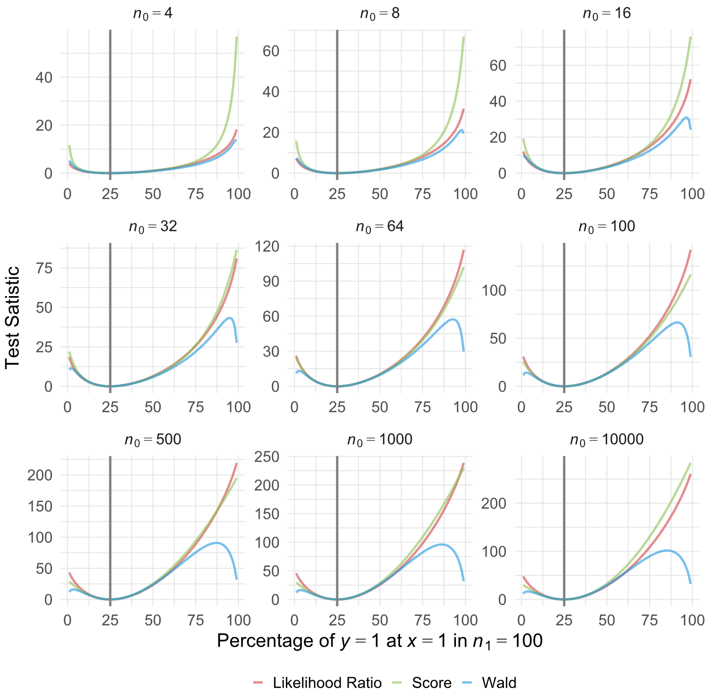
Let's analyze these plots:
- Top-Left (n0=4): With a very small sample size, the test statistics are wildly different. The Wald test (red) behaves erratically, especially at the extremes.
- Moving Right and Down (Increasing Sample Size): As the sample size increases (e.g., to n0=10000 in the bottom-right), notice how the three curves converge and become almost indistinguishable, especially near the center. This is asymptotic equivalence in action.
- Behavior of the Wald Test: Look at the red curve across the plots. It often behaves strangely compared to the others, sometimes dipping below or shooting far above. This visualizes its relative instability. The disagreement between the red curve and the other two is a warning sign about the reliability of the Wald test in those scenarios.
Which Test Should I Use? A Practical Guide
This brings us to the most important question: which test should you use and trust?
How are the likelihood ratio, Wald, and Lagrange multiplier (score ...
The UCLA Statistics FAQ we looked at previously has an excellent summary section that provides practical advice based on the differences we've just discussed.
Please read the section 'A comparison of the three tests'. Focus on the practical recommendations. Note the conclusion that for most situations today, 'we generally recommend running the likelihood ratio test'. Also, pay attention to the specific use cases suggested for the Wald and Score tests.
Synthesizing this information, here is your functional guide:
| Test | When to Use It | What to Watch Out For |
|---|---|---|
| Likelihood Ratio Test (LRT) | The default choice for formal hypothesis testing. Use it when you are testing one or a few pre-specified predictors. It is generally the most powerful and reliable of the three tests. | It's slightly more work as it requires fitting two models (the full and the reduced). However, with modern computers, this is rarely a practical barrier. |
| Wald Test | Quickly inspecting the summary output of a model. Every coefficient in a standard GLM summary table has a z-statistic or t-statistic next to it—that's a Wald test. It's convenient for a first look. | Be cautious if the p-value is borderline (e.g., 0.04 or 0.06). If a key conclusion depends on a borderline Wald test, you should confirm it with an LRT. |
| Score Test | Automated model building and variable selection. When you have hundreds of potential predictors to screen, the Score test is very efficient because it only requires fitting the null model once. You can then test the potential contribution of each new variable without refitting. | It is generally less powerful than the LRT, meaning it might miss some real effects (higher Type II error rate). |
The most critical takeaway: If the Wald test and the Likelihood Ratio Test give you different conclusions for the same hypothesis (i.e., one is significant and the other is not), you should trust the Likelihood Ratio Test. The disagreement itself is a strong indicator that the quadratic approximation used by the Wald test is failing.
Conclusion
You now have a deeper, more functional understanding of the "big three" hypothesis tests in GLMs. You know not only what they do, but why they are different and how to navigate those differences in your own data analysis.
Key Takeaways:
- The Wald, LRT, and Score tests are asymptotically equivalent, meaning they agree in large samples, but can differ in finite samples.
- The LRT and Score tests are invariant to re-parameterization, a key theoretical advantage over the Wald test, which is not.
- The test statistics often follow the inequality Wald ≥ LRT ≥ Score, making the Wald test the most likely to reject the null.
- Disagreements between the tests are a red flag, often indicating small sample sizes or boundary issues, and they reveal the unreliability of the Wald test's underlying assumptions.
- For planned hypothesis tests, the LRT is the recommended 'gold standard', while the Wald test is for quick inspection and the Score test is for efficient variable screening.
Preview of the Next Lesson:
In the next lesson, we will put this knowledge into action. We will learn to interpret the standard output of a fitted GLM. You will see how software packages present coefficient estimates, standard errors, and these very test statistics (usually the Wald test by default), and you'll be fully equipped to understand what they mean and, more importantly, what their limitations are.