Introduction
Hello! In our last lesson, we learned how to use deviance to assess the overall goodness of fit for a Generalized Linear Model (GLM). By comparing the null deviance (from a model with no predictors) to the residual deviance (from our fitted model), we could test the collective significance of all our predictors.
Now, we need to zoom in. While it's useful to know the model as a whole is significant, it's often more important to know which specific predictors are driving the effect. This lesson focuses on hypothesis testing for individual GLM coefficients (). We will explore the three main statistical tests used for this purpose:
- The Wald Test
- The Deviance Test (or Likelihood Ratio Test, LRT)
- The Score Test
While these three tests are equivalent in ordinary linear regression, they are not identical in GLMs. Your goal for this lesson is to understand the intuition behind each test, how it works in practice, and its primary strengths and weaknesses. This will give you the functional knowledge to correctly interpret the output from statistical software and choose the right approach for your analysis.
The Unifying Concept: The Log-Likelihood Function
All three tests are different ways of asking the same fundamental question: "How much evidence do we have against the null hypothesis that a coefficient is zero ()?". They each answer this question by examining the log-likelihood function.
Recall that the log-likelihood function, , measures how probable our observed data is, given a particular value for a model coefficient . We find the "best" coefficient estimate, (the Maximum Likelihood Estimate or MLE), by finding the value of that maximizes this function.
The three tests can be understood visually as measuring the "discrepancy" between the MLE () and the value under the null hypothesis (, which is usually 0) in different ways on the log-likelihood curve.

To get a clear overview of this core idea, let's watch a short video.
Wald test | Likelihood ratio test | Score test
The video 'Wald test | Likelihood ratio test | Score test' from the zedstatistics channel provides an excellent visual and conceptual introduction to how these three tests relate to the log-likelihood function.
Please watch the first part of the video (00:26 to 03:54). Focus on the visual explanation of how each test frames the question of 'extremeness': Horizontal distance between the estimate \hat{\theta} and the null value \theta_0. Vertical distance between the log-likelihood at \hat{\theta} and the log-likelihood at \theta_0. Slope (gradient) of the log-likelihood function at the null value \theta_0.
Now that we have the general intuition, let's examine each test in more detail.
1. The Likelihood Ratio Test (LRT) or Deviance Test
The Likelihood Ratio Test is arguably the most intuitive and robust of the three. It directly uses the concept of deviance that we learned in the previous lesson.
-
Core Idea: The LRT asks: "How much worse does our model fit if we force the coefficient to be zero?" It compares the log-likelihood of the full model (with ) to the reduced model (without ). A large drop in log-likelihood when we remove the predictor is strong evidence that the predictor is important.
-
The Test Statistic: The test statistic is calculated from the log-likelihoods of the two models:
This should look familiar! This is precisely the difference in the deviances between the reduced and full models. This statistic follows a distribution with degrees of freedom equal to the number of parameters removed (in this case, 1).
-
Practical Implementation: You must fit two models: one with the predictor(s) of interest and one without.
Chapter 19 Inference in Logistic Regression
This text provides a concise mathematical definition of the LRT and highlights its key advantages.
Read the section '19.2.1 Likelihood Ratio Test (LRT)'. Focus on the formula for the LR Statistic (\Lambda) and its key advantages: it's independent of model parameterization and easily extends to testing multiple parameters.
Let's see how this is done in practice. The following video demonstrates how to perform an LRT in R to compare nested models.
6.6 Likelihood Ratio Test (LRT) in R
The video 'Likelihood Ratio Test (LRT) in R' from MarinStatsLectures shows the practical workflow for conducting an LRT.
Watch from the beginning to 02:29. Notice how the process involves fitting a full model and a reduced model, then comparing them using the anova() function with test='LRT'.
Pros & Cons of LRT:
- Pro: Generally considered the most reliable of the three tests. It is invariant to re-parameterization (e.g., testing gives the same result as testing ).
- Con: It is the most computationally demanding, as it requires fitting two separate models.
2. The Wald Test
The Wald test is the most common test you'll see in statistical output, typically presented as a z-statistic or t-statistic next to each coefficient.
-
Core Idea: The Wald test asks: "How many standard errors is our estimated coefficient away from zero?" It is based on the assumption that the log-likelihood function is approximately quadratic around the maximum.
-
The Test Statistic: The statistic is simple and should be familiar from linear regression:
This statistic is compared to a standard Normal distribution (a Z-test). Squaring it, , gives a statistic that follows a distribution with 1 degree of freedom. -
Practical Implementation: You only need to fit the full model. The coefficient estimate () and its standard error () are used to compute the test.
Chapter 19 Inference in Logistic Regression
This reading explains the Wald test and, crucially, its significant drawbacks.
Read the section '19.2.4 Wald Test'. Pay close attention to the drawbacks: its dependence on model parameterization and its lower reliability in small samples.
The key weakness of the Wald test is its reliance on the quadratic approximation of the log-likelihood function. When this approximation is poor, the Wald test can be unreliable.
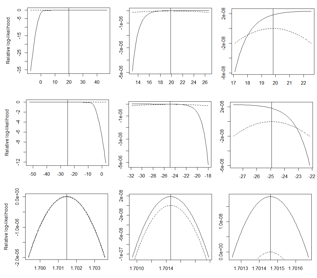
Pros & Cons of Wald Test:
- Pro: Computationally cheap (only requires one model) and easy to interpret. It's the default in most software summaries.
- Con: It is not invariant to re-parameterization. It can perform poorly with small sample sizes or when the true parameter value is far from the null, as the quadratic approximation of the log-likelihood may be inaccurate.
3. The Score Test (or Lagrange Multiplier Test)
The Score test takes a different approach, starting from the null hypothesis.
-
Core Idea: The Score test asks: "If we were at the null hypothesis value (), how steep is the 'slope' of the log-likelihood function?" The slope of the log-likelihood is called the score function. A steep slope suggests that the likelihood would increase substantially if we allowed to be non-zero, providing evidence against the null.
-
The Test Statistic: The formula involves the score function and the information matrix, but the key concept is that it evaluates the gradient at the null value.
-
Practical Implementation: You only need to fit the reduced model (the model without the predictor of interest).
Chapter 19 Inference in Logistic Regression
Finally, let's look at the Score test, also known as the Rao test in some software.
Read the section '19.2.5 Score Test'. Note its main advantage: it only requires fitting the reduced model, making it computationally useful in certain situations.
Pros & Cons of Score Test:
- Pro: Computationally cheap, as it only requires fitting the simpler, reduced model. Like the LRT, it is invariant to re-parameterization. This makes it particularly useful for screening a large number of potential predictors to add to a model (a procedure called forward selection).
- Con: It is generally less powerful than the LRT, especially in smaller samples.
Comparison and Practical Guidance
Now that we've described all three, let's put them together. For large sample sizes, all three tests will give very similar results. However, in finite samples, they can differ.
This final reading provides a fantastic comparison, summarizing what each test does and why you might choose one over another.
How are the likelihood ratio, Wald, and Lagrange multiplier (score ...
The article 'How are the likelihood ratio, Wald, and Lagrange multiplier (score) tests different and/or similar?' from UCLA's statistics consulting group gives a clear, comprehensive comparison.
Please read the section titled 'A comparison of the three tests'. This section masterfully summarizes the differences, the relationship between their test statistics (Wald ≥ LR ≥ Score), and provides practical advice on when to use each test.
Here is a summary table to help consolidate your understanding:
| Feature | Likelihood Ratio Test (LRT) | Wald Test | Score Test |
|---|---|---|---|
| What it Measures | Vertical distance on log-likelihood curve (change in height) | Horizontal distance on log-likelihood curve (distance from null) | Slope of the log-likelihood curve at the null value |
| Models Required | Full AND Reduced | Full ONLY | Reduced ONLY |
| Invariance | Yes, invariant to re-parameterization | No, results can change with re-parameterization | Yes, invariant to re-parameterization |
| Reliability | Generally considered the most reliable and powerful. | Can be unreliable in small samples or with strong effects. | Can be less powerful than LRT, but more reliable than Wald. |
| Best Use Case | Hypothesis testing for one or a few pre-specified predictors. | Quick inspection of coefficients in a model summary. | Screening large numbers of potential predictors to add to a model. |
Conclusion
In this lesson, you've learned about the three fundamental tests for assessing the significance of coefficients in a GLM. You now have the functional understanding to not just read statistical output, but to critically evaluate it.
Key Takeaways:
- The Wald, Likelihood Ratio (LRT), and Score tests are three different ways of testing hypotheses about GLM coefficients by examining the log-likelihood function.
- The LRT (Deviance Test) is generally the most robust method. It compares the fit of nested models and its test statistic is the difference in deviance.
- The Wald Test is the most convenient as it is provided in standard output, but its reliance on a quadratic approximation makes it less reliable in small samples.
- The Score Test is computationally efficient, requiring only the null model, which makes it ideal for variable screening procedures.
- While the tests converge with large samples, for any given analysis, the LRT is often the preferred choice for formal hypothesis testing due to its superior statistical properties.
Preview of the Next Lesson:
We have now described the three main tests. In the next lesson, we will build directly on this foundation to compare their practical and theoretical differences in more depth, looking at situations where their results might diverge and what that tells you about your model and data.