Deviance in GLMs: Understanding Goodness of Fit

From Residuals to Deviance: Generalizing "Goodness of Fit"

In ordinary linear regression, we measure how far our model's predictions are from the actual data by calculating the Residual Sum of Squares:
$\text{RSS}={\sum }_{i=1}^n(Y_i-{\hat{Y}}_i{)}^2$
This works because the errors are assumed to be normally distributed with constant variance. In GLMs, this assumption no longer holds (e.g., for binary or count data, the variance depends on the mean). We need a different way to measure the discrepancy between the observed data and the model's predictions.

The solution is to use the log-likelihood, a concept central to modern statistics. A higher log-likelihood means the model assigns a higher probability to the data we actually observed, indicating a better fit.

To measure how well our model fits, we compare its log-likelihood to the best possible log-likelihood we could ever hope to achieve. This hypothetical "perfect" model is called the saturated model.

Let's watch a video that introduces this crucial concept.

As the video explains, the saturated model perfectly fits the data, giving us a ceiling for model performance. Now we can formally define deviance as the "distance" between our model and this perfect model.

Defining Deviance

Deviance measures the "badness-of-fit" of a GLM by comparing the log-likelihood of our fitted model to the log-likelihood of the saturated model.

To understand this more formally, let's look at a short reading.

The key formula for deviance is:

• $\ell (\text{model})$ is the log-likelihood of our fitted model.
• $\ell (\text{saturated model})$ is the log-likelihood of the perfect, saturated model.

Since the saturated model is the best possible fit, $\ell (\text{model})\le \ell (\text{saturated model})$, which ensures the deviance $D$ is always non-negative. A smaller deviance indicates a better fit, with a deviance of 0 meaning our model is as good as the saturated model.

The multiplication by $-2$ isn't arbitrary; it ensures that the deviance statistic has an approximate chi-squared (${\chi }^2$) distribution under certain conditions, which is extremely useful for hypothesis testing.

The Connection to Linear Regression

You might be wondering how this relates to the RSS you already know. It turns out that deviance is a direct generalization of RSS. For a standard linear model (a GLM with a Normal distribution and identity link), the deviance is exactly equal to the RSS.

This next reading demonstrates this important connection.

This is a powerful idea. Deviance allows us to use a single, consistent framework for measuring error across all kinds of models, from simple linear regression to logistic and Poisson regression.

Null Deviance vs. Residual Deviance

When you fit a GLM in software like R or Python, the summary output typically provides two deviance values: null deviance and residual deviance. Understanding both is key to assessing your model.

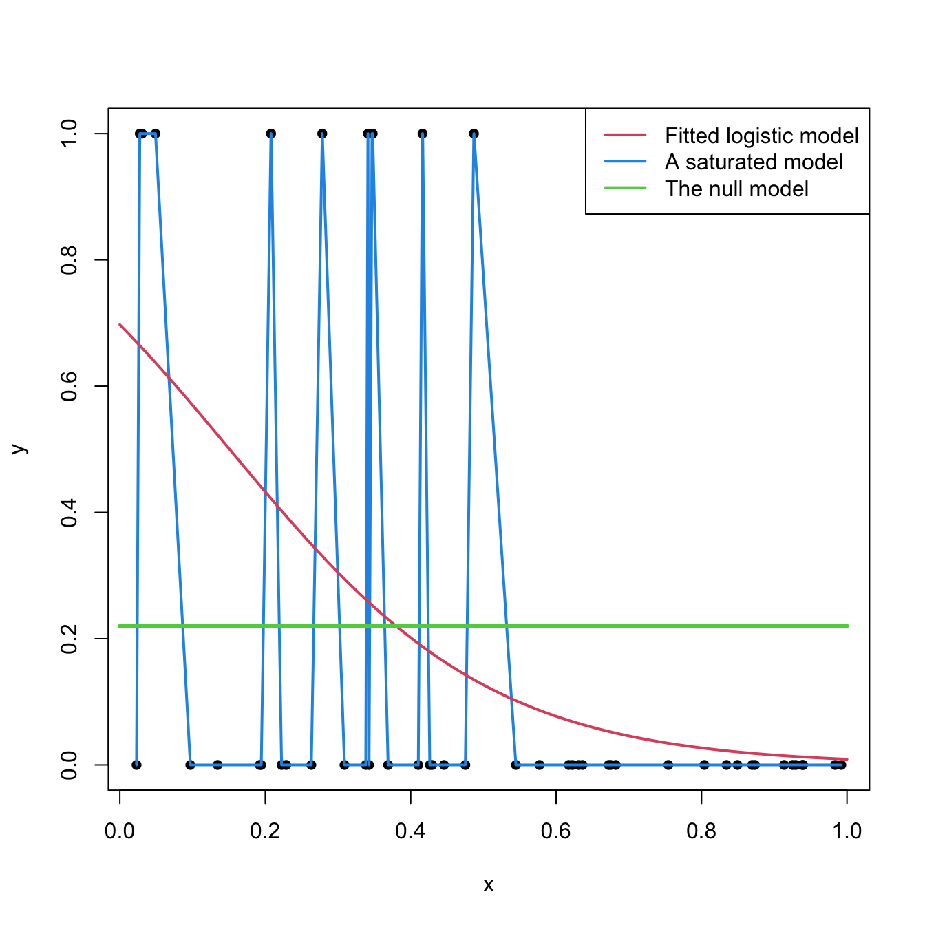
1. Residual Deviance: This is the deviance of your fitted model (the one with predictors). It is analogous to the RSS in linear regression. It tells you how much unexplained variation remains after fitting your model.

2. Null Deviance: This is the deviance of a null model—a model with only an intercept and no predictors. This model predicts the same mean for every observation. The null deviance is analogous to the Total Sum of Squares (SST) in linear regression. It represents the total variation in the data before you've introduced any predictors.

Let's watch the StatQuest video again to get a clear conceptual breakdown of these two types of deviance.

Using Deviance for Goodness-of-Fit Testing

The real power of null and residual deviance comes from comparing them. The difference between them tells you how much the deviance was reduced by including your predictors.

This difference follows a ${\chi }^2$ distribution, with degrees of freedom equal to the number of predictors you added to the model. This allows us to perform a hypothesis test for the overall significance of the model:

• Null Hypothesis (H₀): The predictors in the model are collectively not significant. The reduction in deviance is just due to chance.
• Alternative Hypothesis (H₁): At least one predictor is significant. The model with predictors is a significantly better fit than the null model.

A small p-value (< 0.05) for this test means we can reject the null hypothesis and conclude that our model is a significant improvement over a model with no predictors.

This next resource provides a very practical, step-by-step guide to interpreting these values.

The Pseudo R-squared

Just as you can calculate R-squared in linear regression using SST and RSS, you can calculate a similar metric for GLMs using the null and residual deviances.

$R_{\text{Deviance}}^2=1-\frac{\text{Residual Deviance}}{\text{Null Deviance}}=1-\frac{D}{D_0}$

This is often called a pseudo R-squared. It can be interpreted as the proportion of the deviance explained by the model. While it doesn't have all the same properties as the R-squared from linear regression, it provides a useful heuristic for model fit, ranging from 0 (model is no better than the null) to 1 (model fits perfectly).

To see a final summary and a look at R output, this short video is helpful.

Conclusion

In this lesson, we demystified the concept of deviance and its central role in evaluating GLMs. Building on your knowledge of linear regression, you now have a more general framework for assessing model fit.

Key Takeaways:

• Deviance is the core measure of "badness-of-fit" for a GLM, analogous to the Residual Sum of Squares (RSS) in linear regression.
• It's calculated by comparing the log-likelihood of your fitted model to that of a hypothetical, perfect saturated model.
• Residual Deviance is the deviance of your model with predictors. A smaller value indicates a better fit.
• Null Deviance is the deviance of an intercept-only model and serves as a baseline, analogous to the Total Sum of Squares (SST).
• The difference, Null Deviance - Residual Deviance, can be used in a ${\chi }^2$ test to assess the overall significance of your model's predictors.
• A pseudo R-squared can be calculated from the deviances to estimate the proportion of variation explained by the model.

Preview of the Next Lesson:

We now know how to assess the overall fit of our model. But what about the individual predictors? In our next lesson, we will dive into inference for GLM coefficients. We'll explore the three main statistical tests—the Wald, Deviance (Likelihood Ratio), and Score tests—used to determine whether each predictor has a significant effect on the outcome.